Introduction
Welcome to this informative guide on how to unhide columns in Google Sheets. Google Sheets is a powerful and versatile spreadsheet application that allows you to organize and analyze data effectively. Sometimes, you might find yourself in a situation where you accidentally hide columns or intentionally hide them for better visibility. Whatever the case may be, this guide will walk you through various methods to easily unhide columns and regain access to your valuable data.
Whether you are a beginner or an experienced user of Google Sheets, these methods will help you quickly unhide columns and streamline your workflow. It’s important to note that the steps may vary slightly depending on the version of Google Sheets you are using, but the underlying principles remain the same.
In the following sections, we will explore five different methods to unhide columns in Google Sheets. These methods include using the “View” menu, keyboard shortcuts, the right-click menu, the “Format” menu, and dragging and dropping. Each method offers a simple and efficient way to restore hidden columns in your spreadsheet.
So, without further ado, let’s dive into these methods and get your hidden columns back in no time!
Method 1: Using the “View” Menu
The first method we will explore is using the “View” menu to unhide columns in Google Sheets. This method is straightforward and can be done in just a few simple steps.
To begin, open your Google Sheets spreadsheet and navigate to the top of the screen where you will find the menu options. Click on the “View” menu, and a dropdown menu will appear.
In the dropdown menu, hover your cursor over the “Columns” option. A sub-menu will appear, showing different column-related actions you can perform. Look for the “Hide” option followed by a list of the hidden columns in your spreadsheet.
To unhide a specific column, simply click on the corresponding hidden column. The checkmark next to the column name will disappear, indicating that the column is now visible.
If you want to unhide multiple columns at once, hold down the “Ctrl” key (or “Cmd” key on Mac) and click on each hidden column you want to unhide. The checkmark will disappear for each selected column, indicating that they are now visible.
Alternatively, if you want to unhide all the hidden columns in one go, simply click on the “Unhide all columns” option at the bottom of the sub-menu. This will make all the hidden columns visible again.
Once you have completed the above steps, you will have successfully unhidden the columns using the “View” menu. You can now view and edit the data in the previously hidden columns, allowing you to continue working on your spreadsheet with ease.
Keep in mind that this method works only for columns that have been hidden using the “View” menu. If the columns were hidden using another method, such as by adjusting the column width to zero, you will need to use a different method to unhide them.
Method 2: Using the Keyboard Shortcuts
Another quick and efficient way to unhide columns in Google Sheets is by utilizing keyboard shortcuts. This method allows for speedy column unhiding with just a few key presses.
To begin, open your Google Sheets spreadsheet and make sure that the desired sheet is active and visible. Then, select the first column to the left of the hidden columns. Press and hold the “Shift” key on your keyboard and then press the right arrow key. This action will highlight all the columns to the right, including the hidden ones.
Once the hidden columns are selected, release the “Shift” key. With the columns still selected, press “Ctrl” + “Alt” + “Shift” + “0” (zero) on your keyboard (or “Cmd” + “Option” + “Shift” + “0” on Mac). This keyboard shortcut will unhide the selected columns, making them visible again.
If you want to unhide individual hidden columns using keyboard shortcuts, select the column to the left of the hidden column, then press “Ctrl” + “Shift” + “0” (zero) (or “Cmd” + “Shift” + “0” on Mac).
It’s important to note that the keyboard shortcut for unhiding columns only works if the columns are contiguous (next to each other). If the hidden columns are not contiguous, you will need to use a different method to unhide them.
Using keyboard shortcuts can greatly expedite the process of unhiding columns in Google Sheets. It allows you to quickly select and unhide multiple columns without the need to navigate through menus or sub-menus.
Now that you’re familiar with this method, you can confidently use keyboard shortcuts to unhide columns and enhance your productivity while working with Google Sheets.
Method 3: Using the Right-Click Menu
If you prefer a more intuitive and context-specific approach, you can unhide columns in Google Sheets using the right-click menu. This method allows you to easily unhide individual or multiple columns directly from the spreadsheet.
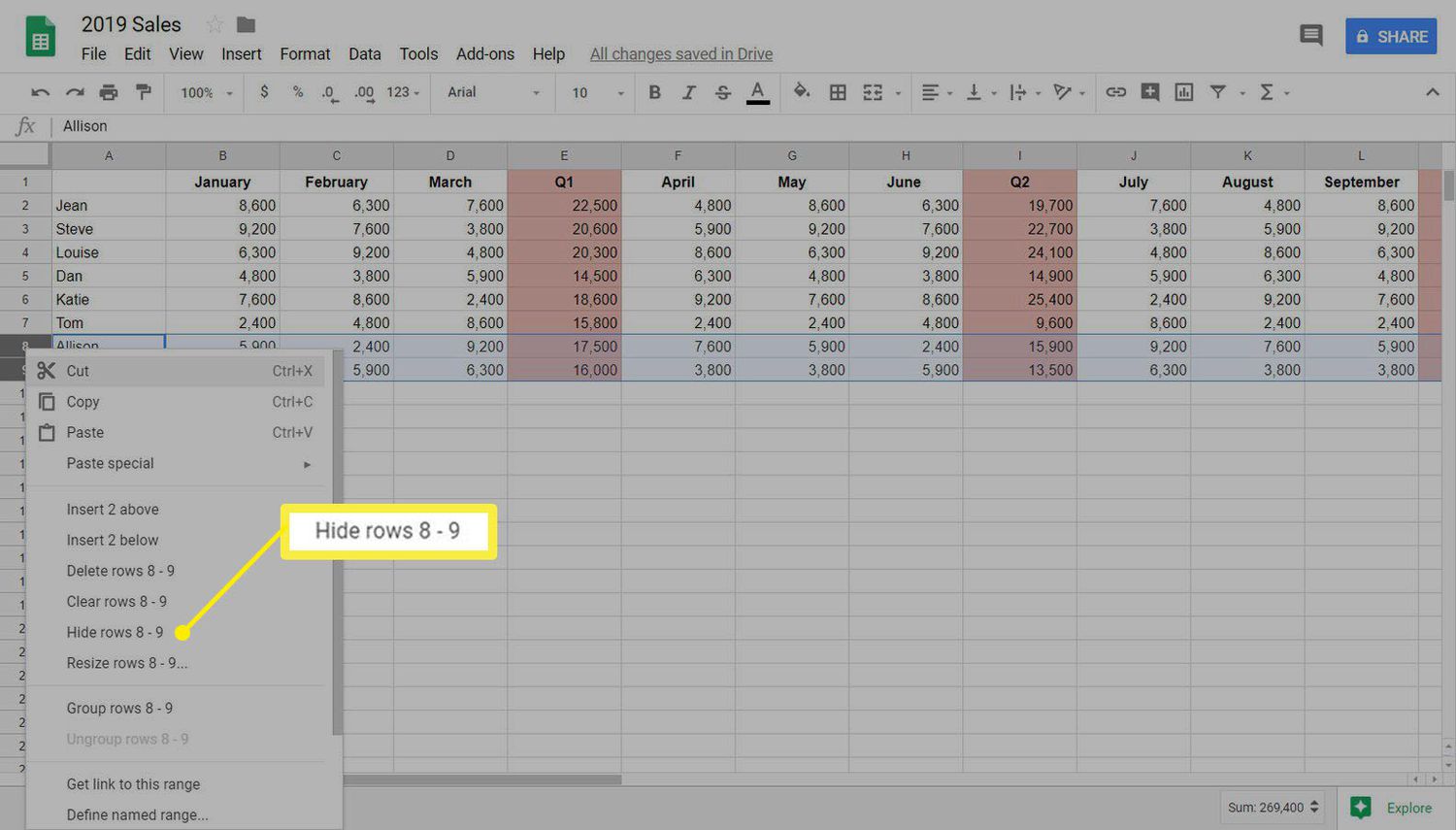
To begin, open your Google Sheets spreadsheet and navigate to the column header area. Right-click on the column header of the first visible column to the left of the hidden column(s). A context menu will appear, displaying various options.
In the context menu, click on the “Unhide Columns” option. This will immediately unhide the hidden column that is adjacent to the column you right-clicked on.
If you want to unhide multiple columns at once, start by right-clicking on the column header of the first visible column to the left of the hidden columns. Then, hold down the “Shift” key on your keyboard and right-click on the column header of the last visible column to the left of the hidden columns. This action will select all the columns in between. Finally, click on the “Unhide Columns” option in the context menu to unhide the selected columns.
Using the right-click menu to unhide columns provides a convenient and visual way to manage hidden columns in Google Sheets. It allows you to easily unhide individual or multiple hidden columns directly from the spreadsheet interface.
Now that you’re familiar with this method, feel free to use the right-click menu in Google Sheets to swiftly unhide your hidden columns and regain access to your data.
Method 4: Using the “Format” Menu
Another effective way to unhide columns in Google Sheets is by utilizing the “Format” menu. This method offers a straightforward approach to unhiding columns with just a few clicks.
To begin, open your Google Sheets spreadsheet and select the columns adjacent to the hidden column(s) that you want to unhide. You can do this by clicking on the first visible column header, holding down the “Shift” key on your keyboard, and then clicking on the last visible column header.
Once the columns are selected, go to the top of the screen and click on the “Format” menu. A dropdown menu will appear with various formatting options.
In the dropdown menu, hover your cursor over the “Column” option. This will expand a submenu with column-related formatting actions.
In the submenu, click on the “Unhide” option. This will immediately unhide the selected columns, making them visible in your spreadsheet once again.
If you want to unhide all the hidden columns at once, without selecting individual columns, you can find the “Unhide” option directly under the “Format” menu. Simply click on it, and all the hidden columns in your spreadsheet will be unhidden instantly.
The “Format” menu provides a simple and convenient method to unhide columns in Google Sheets. It allows you to quickly access the formatting options, including unhiding columns, which can help you manage and organize your spreadsheet effectively.
Now that you’re familiar with this method, you can confidently use the “Format” menu in Google Sheets to easily unhide columns and ensure seamless data visibility in your spreadsheet.
Method 5: Using Dragging and Dropping
If you prefer a more interactive and visual approach, you can unhide columns in Google Sheets by using the dragging and dropping technique. This method allows you to easily restore hidden columns by adjusting their position within the spreadsheet.
To begin, open your Google Sheets spreadsheet and locate the column headers. Look for any visible columns to the left or right of the hidden columns.
Click and hold on the column header of the visible column closest to the hidden columns. Then, drag the column header towards the hidden columns. As you drag the column header closer to the hidden columns, you will notice a blue vertical line appear.
Position the column header on the blue vertical line, indicating the desired position for the hidden columns. Release the mouse button to drop the columns in the new position.
By dragging and dropping the visible column towards the hidden columns, you effectively unhide the previously hidden columns and rearrange the columns in your spreadsheet.
This method is particularly useful when you want to unhide individual columns or when you need to reorganize the columns in a specific order. It provides a visual representation of the column movement, allowing you to have immediate control over the column visibility without relying on menus or shortcuts.
Feel free to experiment with dragging and dropping columns in Google Sheets to unhide hidden columns and customize the layout of your spreadsheet according to your requirements.
Conclusion
Unhiding columns in Google Sheets is a crucial skill for effectively managing and organizing your spreadsheet data. Whether you accidentally hide columns or intentionally hide them for better visibility, knowing how to unhide them quickly can save you time and frustration.
In this guide, we explored five different methods to unhide columns in Google Sheets: using the “View” menu, keyboard shortcuts, the right-click menu, the “Format” menu, and dragging and dropping. Each method offers a simple and efficient way to restore hidden columns, depending on your preference and specific scenario.
The “View” menu provides an easy-to-access option to unhide columns, suitable for both individual and bulk column unhiding. Keyboard shortcuts offer a speedy approach for unhiding columns, ideal for users who prefer utilizing key commands. The right-click menu offers a context-specific method for directly unhiding columns from within the spreadsheet. The “Format” menu provides a straightforward way to manage hidden columns through the selection of formatting options. Lastly, dragging and dropping offers an interactive and visual method to unhide columns while rearranging their position in the spreadsheet.
By familiarizing yourself with these methods, you can confidently unhide columns in Google Sheets and regain access to your hidden data. Remember to choose the method that best suits your needs and preferences for a seamless and efficient workflow.
Now that you have the knowledge and tools to unhide columns in Google Sheets, go ahead and explore the various methods in your own spreadsheets. Unlock the hidden potential of your data and maximize your productivity with Google Sheets.