How To Subtract In Google Sheets

Introduction

Welcome to our comprehensive guide on how to subtract in Google Sheets. Whether you’re a student, professional, or simply someone who wants to organize their data effectively, Google Sheets provides a powerful platform for performing various calculations, including subtraction. In this tutorial, we will walk you through the step-by-step process of subtracting numbers in Google Sheets, from basic subtraction formulas to more advanced techniques to enhance your productivity.

Google Sheets is a web-based spreadsheet program that offers a wide range of features, making it a popular choice for data analysis and management. With its intuitive interface and robust functionality, you can perform complex calculations, manipulate data, and create interactive visualizations, all within a collaborative environment.

Subtraction is a fundamental arithmetic operation that involves finding the difference between two numbers. In Google Sheets, you can subtract numbers using either basic formulas or the built-in functions specifically designed for subtraction. By mastering these techniques, you’ll be able to subtract numbers accurately and efficiently, whether you’re working on a simple budget or performing complex financial analyses.

In this guide, we’ll cover the essential steps to subtract in Google Sheets, including creating a new spreadsheet, entering data, using subtraction formulas, customizing formatting, and troubleshooting common errors. Additionally, we’ll explore advanced concepts such as absolute and relative cell references, as well as time-saving techniques like the AutoSum feature.

So, let’s dive into the wonderful world of subtraction in Google Sheets and discover how this powerful tool can simplify your calculations and improve your productivity.

Step 1: Open Google Sheets and create a new spreadsheet

The first step to subtracting in Google Sheets is to open the application and create a new spreadsheet. To do this, follow these simple instructions:

1. Launch your web browser and navigate to https://www.google.com/sheets.
2. Sign in to your Google account. If you don’t have one, you can create a free account by clicking on the “Create account” button.
3. Once you’re signed in, you’ll be directed to the Google Sheets homepage. Click on the “Blank” option to start a new spreadsheet.
4. A new spreadsheet will open in another tab, displaying a grid of cells.

Google Sheets provides a user-friendly interface that allows for easy navigation and manipulation of data. By creating a new spreadsheet, you’re ready to begin subtracting numbers and performing other calculations.

It’s worth mentioning that Google Sheets also offers various templates for different purposes, such as budgeting, project management, and data analysis. If you prefer to start with a pre-designed template, you can click on the “Template gallery” option when creating a new spreadsheet and choose the one that suits your needs.

Once you have your new spreadsheet open, you’re now ready to move on to the next step: entering your data.

Step 2: Enter your data in the appropriate cells

After creating a new spreadsheet in Google Sheets, the next step is to enter the data that you want to subtract. Follow these steps to enter your data:

1. Select the cell where you want to enter your first number. You can click on the desired cell to select it.
2. Type in the number and press Enter on your keyboard. The number will be entered into the selected cell.
3. Repeat the process for any additional numbers that you want to subtract.

Google Sheets provides a grid-like structure where each cell can store a piece of data, such as numbers, text, or formulas. You can easily navigate between cells using the arrow keys on your keyboard or by clicking on the desired cell.

When entering data, make sure to choose the appropriate cell for each number. If you’re subtracting a series of numbers in a sequential order, you can enter them in a row or column. For non-sequential numbers, you can enter them in any available cells within the spreadsheet.

Keep in mind that Google Sheets allows you to format cells to match the type of data you’re entering. For example, you can format cells as numbers, currencies, dates, or percentages. This formatting can be helpful when subtracting numbers that require specific decimal places or precision.

Once you’ve entered all the numbers you want to subtract, you’re ready to move on to the next step: selecting the cell where you want the subtraction result to appear.

Step 3: Select the cell where you want the subtraction result to appear

After entering the numbers you want to subtract in Google Sheets, it’s time to select the cell where you want the subtraction result to appear. Follow these simple steps to select the desired cell:

1. Click on the cell where you want the subtraction result to be displayed. This will highlight the cell, indicating that it is selected.
2. If the cell is not currently visible on the screen, you can navigate to it by scrolling or using the arrow keys.

Selecting the appropriate cell is essential, as it determines where the subtraction result will be displayed. This allows you to organize your data and calculations in a logical and structured manner.

It’s important to note that the selected cell can be located anywhere within the spreadsheet. For example, you may choose to display the subtraction result in a different row or column than the numbers being subtracted. Google Sheets provides the flexibility to customize your spreadsheet layout according to your specific needs.

Once you have selected the desired cell for the subtraction result, you’re ready to proceed to the next step: using the subtraction formula to perform the calculation.

Step 4: Use the subtraction formula

Now that you have entered your data and selected the cell for the subtraction result in Google Sheets, it’s time to use the subtraction formula to perform the calculation. Follow these steps to subtract numbers using a formula:

1. In the selected cell, type an equals sign (=) to indicate that you’re entering a formula.
2. After the equals sign, type the cell reference for the first number you want to subtract.
3. Next, type a minus sign (-) to represent the subtraction operation.
4. Then, type the cell reference for the second number you want to subtract.
5. Press Enter on your keyboard to apply the formula and display the subtraction result in the selected cell.

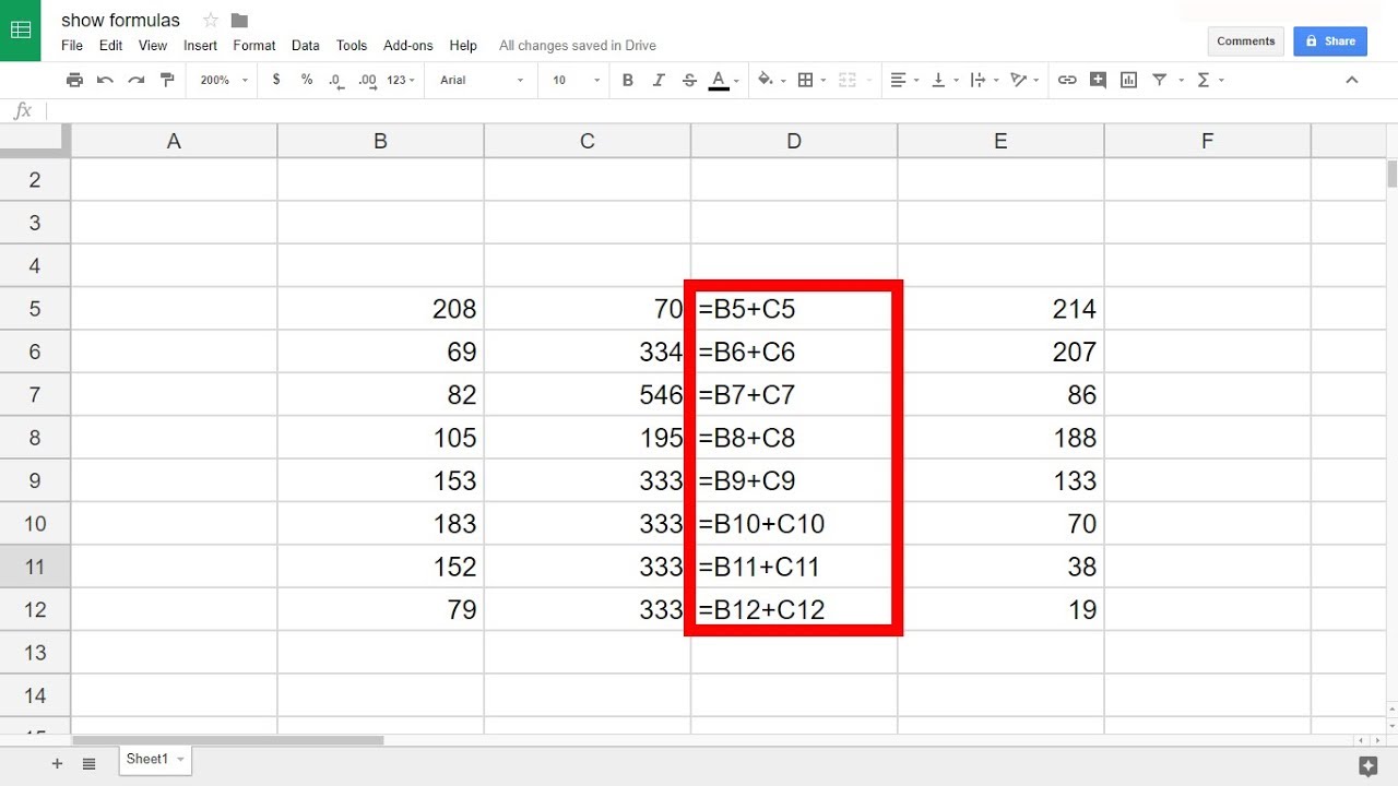
For example, if you want to subtract the number in cell A1 from the number in cell B1, the formula would look like this: =B1 – A1. After pressing Enter, the subtraction result will appear in the selected cell.

Google Sheets allows you to use a combination of cell references, numbers, and mathematical operators to create complex subtraction formulas. You can subtract multiple numbers by simply extending the formula. For example, to subtract the numbers in cells A1, B1, and C1, the formula would look like this: =B1 – A1 – C1.

Additionally, you can use parentheses to control the order of operations in your subtraction formula. For example, if you want to subtract the sum of two numbers from another number, you would enclose the addition operation in parentheses. For example: =A1 – (B1 + C1).

By utilizing subtraction formulas in Google Sheets, you can easily perform intricate calculations and obtain accurate results in seconds.

Step 5: Apply the subtraction formula to multiple cells

In Google Sheets, you can apply the subtraction formula to multiple cells to perform the same subtraction operation across a range of data. This allows you to quickly calculate the differences between corresponding numbers in different cells. Follow these steps to apply the subtraction formula to multiple cells:

1. Select the cell that contains the subtraction formula.
2. Place your cursor on the small square in the bottom right corner of the selected cell. The cursor will change to a plus sign (+).
3. Click and drag the plus sign down or across the cells where you want to apply the formula.
4. Release the mouse button to automatically fill in the subtraction formula in the selected cells.

When you apply the subtraction formula to multiple cells, Google Sheets adjusts the cell references accordingly. For example, if the original formula subtracts values from cells A1 and B1, and you apply it to the cells below, the formula will adjust to subtract values from cells A2 and B2, A3 and B3, and so on.

This feature is particularly useful when you have a large dataset and want to perform the same subtraction operation across multiple rows or columns. It saves you time and effort by automatically copying and adjusting the formula for each corresponding cell.

Moreover, if you need to apply the subtraction formula to a non-contiguous range of cells, you can select all the cells while holding down the Ctrl key (Windows) or Command key (Mac). Then, follow the same steps mentioned above to apply the formula to the selected cells.

By applying the subtraction formula to multiple cells, you can efficiently calculate and compare differences in your data without having to manually enter the formula in each individual cell.

Step 6: Customize the formatting of the subtraction result

After performing the subtraction in Google Sheets, you have the option to customize the formatting of the subtraction result. Formatting allows you to enhance the appearance of the cell and make the result more visually appealing. Follow these steps to customize the formatting of the subtraction result:

1. Select the cell containing the subtraction result.
2. Right-click on the cell and select “Format cells” from the context menu. Alternatively, you can click on the “Format” tab in the top menu and choose “Number” from the dropdown menu.
3. In the “Format cells” or “Number” dialog box, you can choose different formatting options such as number format, decimal places, currency symbol, date format, or percentage.
4. Make your desired formatting selections and click “Apply” or “OK” to apply the formatting changes.

Google Sheets provides a wide range of formatting options to suit your needs. You can choose to display the subtraction result as a general number, a specific currency, a date, a percentage, or any other desired format. Additionally, you can control the number of decimal places shown or add custom symbols such as dollar signs or commas.

Furthermore, you can apply other formatting options such as font styles, font sizes, text alignment, cell borders, cell colors, and more to further customize the appearance of the cell containing the subtraction result. These formatting options can be accessed through the “Format” tab in the top menu of Google Sheets.

By customizing the formatting of the subtraction result, you can present your data in a clear and visually appealing manner, making it easier to interpret and understand.

Step 7: Use the AutoSum feature for quick subtraction

To expedite the subtraction process in Google Sheets, you can utilize the AutoSum feature. The AutoSum feature automatically determines the range of cells to subtract and generates the subtraction formula for you. Follow these steps to use the AutoSum feature for quick subtraction:

1. Select the cell where you want the subtraction result to appear.
2. Click on the “Σ” (Sigma) symbol in the top menu. The AutoSum drop-down menu will appear.
3. In the AutoSum drop-down menu, select “Sum” to subtract the values in the selected range of cells.
4. Google Sheets will automatically determine the range of cells and generate the subtraction formula for you.
5. Press Enter on your keyboard to apply the formula and display the subtraction result.

The AutoSum feature is especially useful when you have a contiguous range of cells that you want to subtract. By using AutoSum, you save time and effort as the formula is applied automatically without any manual input. Additionally, if you need to add further adjustments or modify the subtraction formula, you can edit it after the AutoSum function has been applied.

Furthermore, you can adjust the range of cells that you want to include in the subtraction calculation by clicking on the cell range provided by the AutoSum feature and manually modifying it to match your desired range.

Utilizing the AutoSum feature for quick subtraction not only saves time but also minimizes the chances of errors in your calculations. It allows you to perform repetitive subtractions efficiently, particularly when dealing with large datasets.

Step 8: Use absolute and relative cell references in subtraction formulas

In Google Sheets, you have the flexibility to use both absolute and relative cell references in your subtraction formulas. Understanding the difference between these two types of references is vital for performing accurate calculations. Follow these steps to use absolute and relative cell references in subtraction formulas:

1. When writing a subtraction formula, enter the cell reference for the first number you want to subtract.
2. To use a relative cell reference, simply enter the cell reference without any dollar signs ($). This means that if you copy and paste the formula to another cell, the cell references will adjust automatically based on the relative position of the new cell.
3. To use an absolute cell reference, add a dollar sign ($) before the column letter or row number of the cell reference. This ensures that the cell reference remains fixed when the formula is copied to other cells. You can use a dollar sign before the column letter, the row number, or both, depending on which aspect of the cell reference you want to make absolute.
4. Press Enter on your keyboard to apply the formula and display the subtraction result.

Using relative cell references is useful when you want to perform the same subtraction operation on different rows or columns. As you copy the formula to other cells, the cell references adjust relative to the new location.

On the other hand, using absolute cell references is beneficial when you want to keep a specific cell reference constant, regardless of the location of the formula. This can be helpful when subtracting numbers from a fixed cell, such as a constant or a specific reference point.

To convert a cell reference from relative to absolute or vice versa, you can either manually add or remove the dollar signs, or use the shortcut key combination of F4 to toggle through the different reference modes.

By incorporating absolute and relative cell references in your subtraction formulas, you have more control over how your calculations are performed and can achieve more precise results.

Step 9: Troubleshooting common subtraction formula errors

When working with subtraction formulas in Google Sheets, it’s common to encounter errors. Understanding and resolving these errors is crucial for accurate calculations. Here are some common subtraction formula errors and steps to troubleshoot them:

1. #VALUE! Error: This error occurs when the formula includes non-numeric values or incompatible data types. Double-check that all the cells involved in the subtraction contain valid numerical data.
2. #DIV/0! Error: This error arises when you attempt to divide a cell by zero. Make sure that you’re not dividing any of the numbers in the formula by zero.
3. #REF! Error: This error occurs when a referenced cell in the formula is deleted, causing an invalid cell reference. Ensure that all the referenced cells exist and haven’t been removed or relocated.
4. #NAME? Error: This error occurs when there’s a misspelled function name or an unrecognized term in the formula. Review the formula and verify that all function names and terms are correct.
5. #NUM! Error: This error indicates a numerical error, such as an overflow or an invalid argument. Check for any inconsistencies in the formula or any large numbers that may exceed the calculation limits.

In addition to these specific errors, it’s essential to verify the syntax of the formula, including the correct use of operators, commas, parentheses, and cell references. Google Sheets provides real-time feedback and error indicators that can help pinpoint the location of the error.

If you encounter an error, double-check your formula for any mistakes or inconsistencies. You can also utilize the “Explore” feature in Google Sheets, which offers suggestions and visually analyzes your data to identify potential formula errors.

By troubleshooting and addressing these common subtraction formula errors, you’ll ensure that your calculations in Google Sheets are accurate and reliable.

Conclusion

Congratulations! You’ve reached the end of our comprehensive guide on how to subtract in Google Sheets. We’ve covered all the necessary steps, from creating a new spreadsheet and entering data to using subtraction formulas, customizing formatting, and troubleshooting common errors. By following these steps, you can perform accurate and efficient subtractions in Google Sheets to organize and analyze your data effectively.

Google Sheets offers a powerful platform for performing calculations, including subtraction. Whether you’re a student, professional, or anyone who works with numbers, mastering the art of subtraction in Google Sheets can greatly enhance your productivity and improve your data analysis processes.

Remember, as you work with subtraction formulas, you can further enhance your calculations by utilizing additional features like absolute and relative cell references, AutoSum for quick subtractions, and custom formatting options to make your data more visually appealing.

Should you encounter any errors in your subtraction formulas, be sure to troubleshoot and resolve them promptly. Understanding the common errors, such as #VALUE!, #DIV/0!, #REF!, #NAME?, and #NUM!, will help you spot and correct any issues that may arise.

With this knowledge and practice, you’re equipped to master subtraction in Google Sheets and harness its full potential for your data analysis needs. So, go ahead and start exploring the world of subtraction in Google Sheets, and discover how this versatile tool can streamline your calculations and empower your decision-making process.