Introduction
Welcome to the world of machine learning! In this exciting field, training a model is a crucial step that allows a machine to learn from data and make predictions or decisions. Whether you’re interested in image recognition, natural language processing, or predictive analytics, understanding how to train a model is essential.
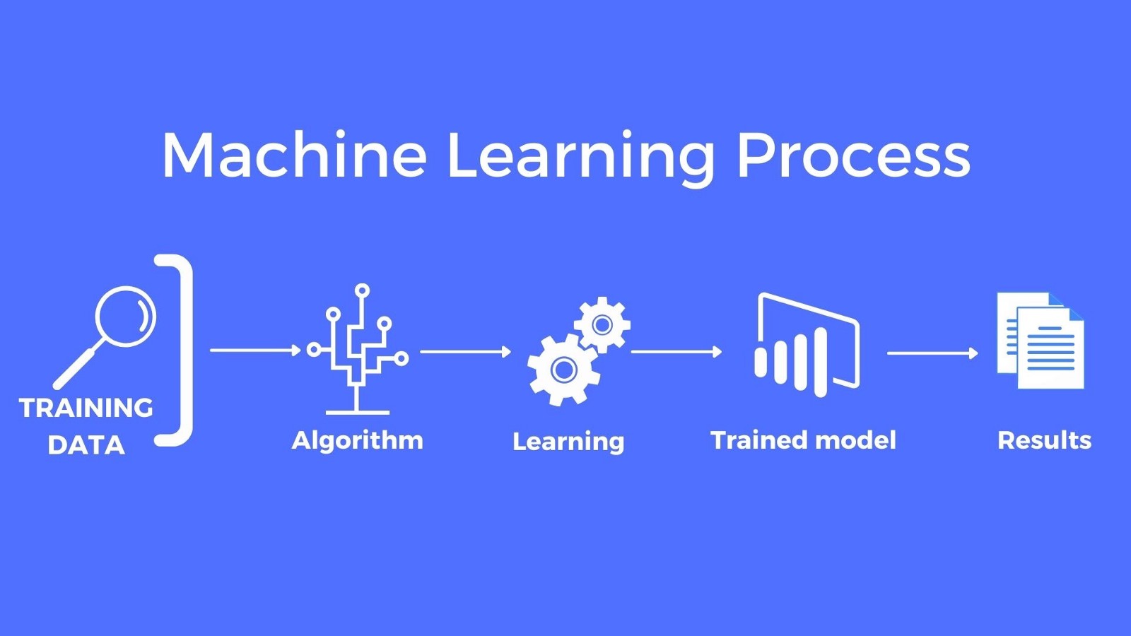
So, what does it mean to train a model in machine learning? Essentially, it involves providing the algorithm with a dataset and allowing it to learn patterns, relationships, and insights from the data. This process enables the model to generalize and make accurate predictions or classifications on new, unseen data.
The heart of training a model lies in data – the more high-quality and diverse the data, the better the model’s performance. However, training a model is not only about feeding it raw data. It often requires preprocessing, choosing the right algorithm, splitting the data into training and testing sets, evaluating performance, and fine-tuning hyperparameters.
Training a model is a complex process, but it’s also a fascinating journey of discovery and optimization. It involves iterative cycles of adjusting parameters, learning from mistakes, and refining the model’s performance.
Throughout this article, we will explore the various steps involved in training a machine learning model, including the importance of data, preprocessing techniques, selecting training algorithms, performance evaluation, and hyperparameter tuning. By the end, you’ll have a clear understanding of how to train a model effectively and how it plays a pivotal role in the field of machine learning.
Definition of Training in Machine Learning
In the realm of machine learning, training refers to the process of teaching a model to recognize patterns, make predictions, or classify data based on a given set of examples or training data. It is a fundamental step in the machine learning pipeline that enables the model to learn and improve its performance over time.
During the training phase, the model is presented with a dataset that consists of input features and corresponding output labels. These inputs and labels form the building blocks for the model to learn the underlying patterns and relationships within the data. The model then adjusts its internal parameters or weights based on the examples provided, aiming to minimize the difference between its predicted outputs and the true labels.
Training a model involves a two-step process: forward propagation and backward propagation. In the forward propagation step, the model takes the input data, applies the learned weights, and produces a predicted output. This output is then compared to the ground truth label using a predefined loss function, which measures the dissimilarity between the predicted and actual values.
In the backward propagation step, also known as backpropagation, the model calculates the gradients of the loss function with respect to each weight. These gradients indicate the direction and magnitude of the weight adjustments required to reduce the loss. The model then uses an optimization algorithm, such as gradient descent, to update the weights iteratively and minimize the loss as it progresses through the training process.
The goal of training a model is to achieve optimal performance on unseen data by generalizing well from the training examples. A well-trained model can effectively make accurate predictions or classifications not only on the training data but also on new, unseen data.
Training a model in machine learning is an iterative process that involves fine-tuning the model’s parameters, exploring different algorithms, and refining the training strategy. It requires careful consideration of various factors, including the quality of the training data, the complexity of the problem, and the available computational resources.
Now that we have a solid understanding of what training entails in machine learning, let’s dive deeper into the role of data in the training process.
The Role of Data in Training a Model
Data is the lifeblood of machine learning, and it plays a critical role in training a model. The quality, quantity, and diversity of the data used for training directly impact the model’s performance and ability to generalize well.
High-quality data is essential for training a model that can make accurate predictions or classifications. This means ensuring that the data is accurate, reliable, and representative of the problem at hand. If the training data contains errors or inconsistencies, it can lead to biased or incorrect predictions.
Another crucial aspect of training data is its quantity. Generally, having a larger training dataset allows the model to learn a more robust representation of the underlying patterns and relationships. With more data, the model can capture a broader range of scenarios and improve its generalization capabilities. However, it’s important to strike a balance, as having too much data can also introduce noise and increase the computational requirements of the training process.
Diversity in the training data is vital for building a model that can handle different scenarios and generalize well. A diverse dataset encompasses various examples, capturing different variations, contexts, and edge cases of the problem. By exposing the model to diverse data, it can learn more nuanced patterns and avoid overfitting to specific instances in the training set.
Preparing the data for training is equally important. This involves cleaning the data, handling missing values, scaling features, and encoding categorical variables. Data preprocessing techniques ensure that the data is in a suitable format for the model to learn from and allows for more meaningful and accurate training.
When training a model, it’s crucial to split the available data into two subsets: the training set and the testing set. The training set is used to teach the model to learn from the data, while the testing set evaluates the model’s performance on unseen data. This separation helps assess the model’s ability to generalize beyond the training data and detect overfitting or underfitting issues.
In summary, data plays a pivotal role in training a machine learning model. The quality, quantity, and diversity of the training data directly impact the model’s performance and generalization abilities. Properly preparing and preprocessing the data, along with careful consideration of training and testing set separation, are crucial steps in training a model that can make accurate predictions on unseen data.
Preprocessing Data for Training
Data preprocessing is a critical step in training a machine learning model. It involves transforming and preparing the raw data to improve the model’s performance and ensure meaningful and accurate training.
One common preprocessing technique is data cleaning, which involves handling missing values, outliers, and errors in the dataset. Missing values can be filled or imputed using various methods, such as mean imputation, median imputation, or regression-based imputation. Outliers can be detected and either removed or treated separately to avoid skewing the model’s training.
Scaling features is another important preprocessing step. Many machine learning algorithms perform better when the features are on a similar scale. Common scaling methods include normalization and standardization. Normalization brings the values of each feature to a similar range, often between 0 and 1. Standardization transforms the data to have a mean of 0 and a standard deviation of 1. The choice of scaling method depends on the nature of the data and the requirements of the specific algorithm being used.
Encoding categorical variables is necessary when dealing with non-numeric data in the training process. Categorical variables, such as gender or product categories, need to be converted into numerical representations that the model can understand. One-hot encoding is a common method where each category is represented by a binary vector, with a 1 indicating the presence of the category and 0 otherwise.
Feature selection or dimensionality reduction is another preprocessing technique that helps improve training efficiency and mitigate the curse of dimensionality. It involves selecting a subset of relevant features or transforming the original features into a lower-dimensional representation. Techniques like Principal Component Analysis (PCA) and feature importance analysis can guide the selection process.
Handling imbalanced classes is important when training models on datasets where one class is significantly more prevalent than the others. In such cases, models tend to favor the majority class, leading to biased predictions. Techniques such as oversampling the minority class, undersampling the majority class, or using synthetic data generation methods like SMOTE (Synthetic Minority Over-sampling Technique) can help address the issue and balance the class distribution for better training outcomes.
Effective data preprocessing ensures that the input data is in a suitable format for the model to learn from. It helps improve the model’s performance, enhance training efficiency, and minimize bias or noise in the training process. By preparing the data carefully, we set the foundation for the model to learn and generalize well to unseen data.
Selecting a Training Algorithm
Choosing the right training algorithm is a crucial step in training a machine learning model. Different algorithms have different strengths, weaknesses, and assumptions, making it important to select the most suitable one for the given problem.
The selection of a training algorithm depends on various factors such as the type of data, the complexity of the problem, the desired output, and the available computational resources. Here are a few common algorithms used in machine learning:
1. Linear Regression: This algorithm is used for regression problems, where the goal is to predict a continuous numerical value. It models the relationship between the input features and the output using a linear equation, aiming to minimize the difference between the predicted and actual values.
2. Logistic Regression: Logistic regression is commonly used for binary classification problems, where the output is a binary value (e.g., yes or no). It models the probability of an input belonging to a certain class using a logistic function.
3. Support Vector Machines (SVM): SVM is a versatile algorithm that can be used for both classification and regression tasks. It finds a hyperplane that separates the input data points into different classes, maximizing the margin between the classes.
4. Random Forest: Random forest is an ensemble learning algorithm that combines multiple decision trees to make predictions. It is effective for both classification and regression tasks and can handle complex interactions and non-linear relationships in the data.
5. Artificial Neural Networks (ANN): ANN is a powerful algorithm inspired by the human brain. It consists of interconnected nodes (neurons) that process and transmit information. Deep learning, a subset of ANN, involves training neural networks with multiple hidden layers to learn hierarchical representations of the data.
6. Gradient Boosting: Gradient boosting is an ensemble learning technique that combines multiple weak learners (typically decision trees) to create a strong predictive model. It trains the learners sequentially, with each subsequent learner correcting the mistakes of the previous ones.
These are just a few examples of the many algorithms available for training a machine learning model. The choice of algorithm depends on various factors such as the nature of the problem, the size of the dataset, the interpretability of the results, and the trade-offs between accuracy, computational complexity, and training time.
It’s important to experiment with different algorithms, analyze their performance, and iterate on the training process to find the best fit for the specific problem at hand. Understanding the strengths and limitations of different algorithms will help in selecting the most appropriate one and maximize the model’s predictive power.
Splitting the Data into Training and Testing Sets
When training a machine learning model, it is crucial to evaluate its performance on unseen data to assess its ability to generalize. This is where the concept of splitting the data into training and testing sets comes into play.
The dataset used for training is typically split into two subsets: the training set and the testing set. The training set is used to teach the model the patterns and relationships present in the data. It guides the model to learn from the examples and adjust its internal parameters or weights accordingly.
On the other hand, the testing set is used to evaluate the performance of the trained model. It contains examples that the model has never seen before, allowing us to assess how well the model generalizes to new, unseen data. By measuring the model’s performance on the testing set, we can gauge its ability to make accurate predictions in real-world scenarios.
There are different approaches to splitting the data into training and testing sets:
1. Holdout Method: In this approach, a fixed percentage of the dataset, typically around 80%, is used for training, while the remaining 20% is reserved for testing. The data is randomly split to ensure that both sets are representative of the overall dataset.
2. Cross-Validation: Cross-validation is a technique that mitigates the variability in performance estimates caused by the randomness of the data split in the holdout method. It involves dividing the data into multiple subsets or “folds” and training the model on different combinations of the folds. This provides a more robust evaluation of the model’s performance.
3. Stratified Sampling: Stratified sampling is used when the dataset is imbalanced, meaning that one class is more prevalent than the others. It ensures that the training and testing sets maintain the same class distribution as the original dataset. This is particularly important to ensure unbiased evaluation in such scenarios.
The size of the testing set depends on the available data and the desired evaluation accuracy. A common practice is to allocate 70-80% of the data for training and the remaining 20-30% for testing. However, the specific split ratio can vary depending on the problem and the size of the dataset.
It is important to note that the testing set should only be used for evaluating the final performance of the model. In the training process, it is essential to avoid peeking or using any information from the testing set to make adjustments to the model. This ensures an unbiased assessment of the model’s generalization ability.
In summary, splitting the data into training and testing sets is a vital step in training a machine learning model. It allows for unbiased evaluation of the model’s performance on unseen data. By carefully partitioning the data and using appropriate evaluation techniques, we can assess the model’s ability to generalize and make accurate predictions in real-world scenarios.
Choosing Performance Measures for Training
When training a machine learning model, it is essential to select appropriate performance measures to evaluate and monitor the model’s performance. These measures provide quantitative insights into how well the model is learning from the training data and making predictions.
The choice of performance measures depends on the nature of the problem and the type of machine learning algorithm being used. Here are a few common performance measures:
1. Accuracy: Accuracy is one of the most widely used performance measures and represents the percentage of correctly predicted instances out of the total number of instances. It is suitable for balanced datasets but can be misleading for imbalanced datasets where the majority class dominates the accuracy metric.
2. Precision and Recall: Precision and recall are performance measures commonly used when dealing with imbalanced datasets and binary classification problems. Precision measures the proportion of correctly predicted positive instances out of all predicted positive instances. Recall measures the proportion of correctly predicted positive instances out of all actual positive instances. These measures help assess the model’s ability to correctly identify positive instances.
3. F1 Score: The F1 score is the harmonic mean of precision and recall. It combines both measures to provide a balanced evaluation of the model’s performance. The F1 score is particularly useful in situations where both precision and recall are important, such as in medical diagnosis or fraud detection.
4. Mean Absolute Error (MAE) and Root Mean Squared Error (RMSE): These measures are commonly used in regression problems to evaluate the difference between the predicted and actual numerical values. MAE represents the average absolute difference between the predicted and actual values, while RMSE represents the square root of the average of the squared differences. These measures provide insights into the model’s ability to estimate continuous variables.
5. Receiver Operating Characteristic (ROC) curve and Area Under the Curve (AUC): ROC curves are commonly used for binary classification problems. They illustrate the trade-off between true positive rate (sensitivity) and false positive rate (1 – specificity) at various classification thresholds. AUC represents the area under the ROC curve and provides a single numerical value that summarizes the overall performance of the model. Higher AUC values indicate better classification performance.
It is important to choose performance measures that align with the specific problem and the desired evaluation criteria. In some cases, a single measure may not be sufficient to capture the entire performance picture. Hence, it is common to consider a combination of multiple measures to obtain a comprehensive evaluation of the model’s performance.
Additionally, it is crucial to interpret performance measures in the context of the problem domain. Evaluating the model’s performance solely based on numerical metrics may not be enough. It is often necessary to consider other factors, such as business requirements, cost constraints, or domain-specific considerations, to make informed decisions about the model’s performance.
By carefully selecting and monitoring performance measures, we can assess the model’s learning progress, identify areas for improvement, and validate the effectiveness of the training process.
Hyperparameter Tuning for Training
Hyperparameters are parameters that are not learned by the model during the training process but are set before training begins. They have a significant impact on the performance and behavior of the machine learning model. Optimizing these hyperparameters is known as hyperparameter tuning and plays a vital role in improving the performance of the trained model.
Hyperparameters can include parameters such as learning rate, regularization strength, number of hidden layers or nodes in a neural network, kernel type in support vector machines, or the number of decision trees in a random forest. These values govern the behavior and complexity of the model, and finding the optimal values can lead to improved performance.
Choosing appropriate hyperparameter values can be challenging, as there is no one-size-fits-all approach. Each problem and dataset may require different hyperparameter configurations to achieve the best performance. Here are a few common techniques used for hyperparameter tuning:
1. Grid Search: Grid search involves creating a predefined grid of possible hyperparameter values and evaluating the model’s performance for each combination. It exhaustively searches through all possible hyperparameter values to find the optimal set that yields the best performance.
2. Random Search: Random search involves randomly sampling hyperparameter values from predefined ranges. It is a less computationally expensive approach than grid search, as it does not evaluate all possible combinations. Instead, it focuses on exploring different regions of the hyperparameter space.
3. Bayesian Optimization: Bayesian optimization is a more advanced technique that uses probabilistic models to optimize the hyperparameters. It starts with an initial set of hyperparameters and uses the performance feedback to guide the search process. Bayesian optimization is particularly effective when the evaluation of each set of hyperparameters is computationally expensive.
4. Genetic Algorithms: Genetic algorithms are inspired by biological evolution and use a population-based approach. Hyperparameter values are represented as individuals in a population, and they evolve over generations through selection, crossover, and mutation. Genetic algorithms can explore complex search spaces and find good hyperparameter configurations.
It is essential to properly validate the performance of the model on a separate validation set during hyperparameter tuning. This prevents overfitting to the training set and ensures that the optimal hyperparameter values generalize well to unseen data.
Automated hyperparameter optimization tools, such as scikit-learn’s GridSearchCV and RandomizedSearchCV or specialized libraries like Optuna and Hyperopt, can streamline the hyperparameter tuning process and efficiently search for the best hyperparameter values.
Hyperparameter tuning can significantly enhance the performance of a trained model. By systematically exploring different hyperparameter configurations and optimizing their values, we can fine-tune the model to achieve better accuracy, improved generalization, and ultimately, more robust predictions on new, unseen data.
Training a Model: Step-by-Step Process
Training a machine learning model involves several key steps that are essential for building an effective and accurate model. Here is a step-by-step process for training a model:
1. Define the Problem: Clearly define the problem you are trying to solve. Determine whether it is a classification, regression, clustering, or other type of problem. Understand the desired outcome and the target performance metrics.
2. Gather and Preprocess the Data: Collect the relevant data for training the model. Make sure the data is representative, clean, and properly formatted. Perform necessary preprocessing steps such as data cleaning, handling missing values, scaling features, and encoding categorical variables.
3. Split the Data: Split the dataset into training and testing sets. Typically, around 70-80% of the data is used for training, while the remaining 20-30% is reserved for testing. Ensure that the split maintains the original distribution of classes or labels, especially for imbalanced datasets.
4. Select an Algorithm: Choose an appropriate algorithm that suits the problem at hand. Consider factors such as the nature of the data, the available computational resources, and the desired level of interpretability. Experiment with different algorithms to find the best fit.
5. Initialize and Train the Model: Initialize the model with suitable hyperparameter values. Feed the training data into the model and optimize the internal parameters using an optimization technique such as gradient descent. Iterate through multiple epochs or iterations, continuously updating the model’s parameters to minimize the loss or error.
6. Evaluate the Model: Evaluate the trained model on the testing data to assess its performance. Calculate relevant performance measures, such as accuracy, precision, recall, or mean squared error, depending on the problem type. Compare the model’s predictions with the true labels or values to understand its effectiveness.
7. Tune Hyperparameters: Fine-tune the model’s hyperparameters to optimize its performance. Utilize techniques like grid search, random search, Bayesian optimization, or genetic algorithms to explore different hyperparameter values and find the best combination. Evaluate the model’s performance at each iteration to guide the hyperparameter tuning process.
8. Iterate and Refine: Analyze the model’s performance and iteratively refine it. Explore alternative algorithms, feature engineering techniques, or data preprocessing strategies to further improve the model’s accuracy or efficiency. Continuously evaluate the model’s performance on new, unseen data to ensure its robustness.
9. Deploy and Monitor: Once satisfied with the model’s performance, deploy it into a production environment. Monitor its performance and gather feedback from real-world inputs. Periodically retrain the model or adapt it as new data becomes available to maintain its accuracy and relevance.
Following these steps will guide you through the process of training a machine learning model effectively. As with any iterative process, be prepared to experiment, learn, and adapt to achieve the best possible outcomes.
Evaluating the Performance of the Trained Model
Evaluating the performance of a trained model is essential to assess its accuracy, reliability, and generalization capabilities. Through proper evaluation, we can gain insights into how well the model performs on new, unseen data and determine its effectiveness in solving the problem at hand. Here are some key aspects to consider when evaluating the performance of a trained model:
1. Performance Metrics: Select appropriate performance metrics based on the problem type. For classification tasks, metrics such as accuracy, precision, recall, and F1 score can be useful. For regression problems, metrics such as mean absolute error (MAE), root mean squared error (RMSE), and R-squared are commonly used. These metrics provide quantitative measures of the model’s performance.
2. Confusion Matrix: For classification problems, a confusion matrix provides a detailed evaluation of the model’s predictions. It displays the counts of true positives, true negatives, false positives, and false negatives. From the confusion matrix, metrics such as precision, recall, and accuracy can be derived.
3. Cross-Validation: Perform cross-validation to obtain a more robust evaluation of the model. Split the data into multiple subsets or folds and train the model on various combinations of these folds. This helps assess the model’s performance across different subsets of the data and mitigates the impact of random variations in the split.
4. Overfitting and Underfitting Assessment: Check for signs of overfitting or underfitting during evaluation. Overfitting occurs when the model performs well on the training data but fails to generalize to new data. Underfitting, on the other hand, indicates that the model’s complexity is insufficient to capture the underlying patterns in the data. Identifying and addressing these issues is crucial to improving the model’s performance.
5. Visualizations: Utilize visualizations to gain a deeper understanding of the model’s performance. Visualize the predicted outcomes against the actual outcomes through scatter plots, histograms, or line graphs. Visualizations can reveal patterns, outliers, or areas where the model struggles to make accurate predictions.
6. Domain Expertise: Consider domain knowledge and expert insight while evaluating the model’s performance. It is essential to interpret the results within the context of the problem domain and understand the practical implications of the model’s predictions. Domain experts can provide valuable feedback on the model’s performance and suggest improvements or additional evaluation criteria.
7. Comparison with Baselines: Compare the performance of the trained model with baseline models or previous iterations to gauge progress. Baselines can be simple rule-based models or initial implementations of the model. By comparing against these benchmarks, we can evaluate the incremental improvement achieved through training.
Through a comprehensive evaluation process, we gain a holistic understanding of the model’s effectiveness and limitations. Evaluation allows us to make informed decisions about the model’s deployment, iterate on the training process, or consider alternative approaches if needed. Continuous evaluation and monitoring are crucial to ensure the model remains accurate and aligned with the evolving requirements of the problem domain.
Conclusion
Training a model in machine learning is a multi-step process that involves preparing the data, selecting a suitable algorithm, splitting the data into training and testing sets, choosing performance measures, tuning hyperparameters, and continuously evaluating the model’s performance. Each step contributes to building an accurate and reliable model that can make predictions or classifications on new, unseen data.
The role of data cannot be overstated in training a model. High-quality, diverse, and well-preprocessed data lays the foundation for the model to learn meaningful patterns and relationships. Selecting the right algorithm is crucial, as different algorithms have different strengths and assumptions. Properly splitting the data into training and testing sets ensures unbiased evaluation of the model’s performance.
Choosing appropriate performance measures provides quantitative insights into how well the model is performing. Hyperparameter tuning optimizes the model’s performance by refining the values that control its behavior. Evaluating the performance of the trained model involves assessing metrics, using techniques like cross-validation, and visualizing the results.
Throughout the training process, it is essential to iterate, refine, and adapt based on the evaluation feedback. Models should be continuously monitored and updated to maintain accuracy and relevance in real-world scenarios. The ultimate goal is to deploy a well-trained model that can make accurate predictions or decisions and drive valuable insights and actions.
Training a model in machine learning requires a combination of technical knowledge, analytical skills, and creativity. It is a dynamic and iterative process, where understanding the problem domain, selecting appropriate techniques, and interpreting and evaluating results are key factors for success.
As the field of machine learning continues to evolve, the training process will become more sophisticated. New algorithms, advanced preprocessing techniques, and automated tools for hyperparameter tuning will emerge. Staying updated with the latest developments and continuously honing our skills will allow us to build more powerful and effective machine learning models.


