Introduction
Welcome to the world of machine learning! As technology continues to evolve, machine learning has emerged as a powerful tool in various industries, including finance, healthcare, and marketing. With the ability to analyze complex data and make accurate predictions, machine learning models have revolutionized decision-making processes and automated tasks that were once considered impossible.
However, with the wide range of machine learning algorithms available, choosing the right model for a specific task can be a daunting challenge. This is where the process of comparing machine learning models becomes crucial. By comparing and evaluating different models, we can identify the most suitable one to achieve our desired outcomes.
Comparing machine learning models involves examining their performance, accuracy, and ability to generalize to new, unseen data. It helps us understand the strengths and weaknesses of each model, enabling us to make informed decisions about which one to choose.
In this article, we will explore the essential steps and considerations for comparing machine learning models. We will delve into the evaluation metrics used to assess model performance, the importance of data preprocessing, splitting data into training and testing sets, and the training and fine-tuning of models.
Furthermore, we will discuss the significance of evaluating models using various metrics, including accuracy, precision, recall, f1-score, and area under the receiver operating characteristic curve (AUC-ROC). By understanding these evaluation metrics and comparing models based on their performance, we can gain valuable insights and make data-driven decisions.
Importantly, we will also address the importance of considering algorithm complexity and interpretability. While some models may achieve higher accuracy, they may also be more complex and difficult to interpret, making them less suitable for certain applications. We will explore how these factors play a role in choosing the best model.
Finally, we will discuss the visualization of results, which can aid in understanding and interpreting model performance. We will explore various visual techniques, such as confusion matrices, ROC curves, and precision-recall curves, to gain a comprehensive understanding of how different models compare.
By the end of this article, you will have a clear understanding of the importance of comparing machine learning models and the steps involved in making an informed decision. So, let’s dive in and unravel the world of model comparison!
Understanding the Importance of Comparing Machine Learning Models
When it comes to implementing machine learning in real-world scenarios, the choice of model can significantly impact the success of the solution. Each machine learning algorithm has its own set of assumptions, strengths, and limitations. Therefore, it is crucial to compare multiple models to identify the best fit for a particular task.
One of the primary reasons for comparing machine learning models is to evaluate their performance. By comparing metrics such as accuracy, precision, recall, and F1-score, we can assess how well a model is able to classify or predict outcomes. This evaluation is essential in determining which model is the most accurate and reliable.
Additionally, comparing models helps us understand the generalization capabilities of each algorithm. It is crucial to ensure that our models can perform well on unseen data. By evaluating the performance on a testing set that was not used during the model training phase, we can assess how well a model can adapt to new and unknown data. This is a critical aspect of real-world applications.
Another reason to compare machine learning models is to gain insights into their strengths and weaknesses. Some models may excel at handling imbalanced datasets, while others may perform better with high-dimensional data. By comparing models, we can determine which ones are better suited for specific data characteristics.
Moreover, comparing machine learning models provides an opportunity to assess computational complexity. While achieving high accuracy is essential, it is equally important to consider the efficiency and scalability of models. Comparing models can help us understand their computational requirements, allowing us to choose models that strike the right balance between accuracy and efficiency.
Furthermore, interpreting models is crucial in many applications, especially those that involve making decisions based on the model’s outputs. Some models, such as decision trees, provide transparent rules that can be easily understood by humans. In contrast, neural networks and deep learning models may offer higher accuracy but lack interpretability. By comparing the interpretability of different models, we can choose the one that aligns with our requirements.
Overall, comparing machine learning models enables us to make well-informed decisions based on empirical evidence and objective evaluation. It helps us understand the trade-offs between accuracy, generalization, computational complexity, and interpretability. By comparing and evaluating multiple models, we can choose the best model for our specific task, leading to improved performance and better outcomes.
Choosing the Right Evaluation Metrics
When comparing machine learning models, selecting the appropriate evaluation metrics is crucial as it determines how we measure and quantify the performance of each model. The choice of evaluation metrics depends on the nature of the problem we are trying to solve and the specific goals we want to achieve.
One commonly used evaluation metric is accuracy, which measures the percentage of correctly classified instances. While accuracy provides a good measure of overall model performance, it may not be suitable for imbalanced datasets, where the number of instances in each class is significantly different. In such cases, metrics like precision, recall, and F1-score are more informative.
Precision measures the proportion of true positive predictions out of all positive predictions, highlighting the model’s ability to avoid false positive errors. Recall, on the other hand, measures the proportion of true positive predictions out of all actual positive instances, emphasizing the model’s ability to find all positive instances. The F1-score combines precision and recall into a single metric, providing a balanced measure of model performance.
In some cases, we might encounter problems where correctly identifying one class is more important than the others. For instance, in a medical diagnosis scenario, correctly identifying a life-threatening condition is more critical than correctly identifying a less severe condition. In such cases, we can use metrics like the area under the receiver operating characteristic curve (AUC-ROC) to evaluate model performance. This metric considers the trade-off between true positive rate and false positive rate and provides an overall measure of discrimination power.
Choosing the right evaluation metric also depends on the specific domain and the problem at hand. For instance, in recommendation systems, metrics like precision at K or average precision can be used to evaluate the relevance of recommended items to users. Mean squared error (MSE) or root mean squared error (RMSE) are common evaluation metrics for regression problems that measure the average squared difference between predicted and actual values.
It is important to note that there is no one-size-fits-all evaluation metric. The choice of metrics should align with the specific requirements of the problem and the preferences of stakeholders. By carefully selecting the appropriate evaluation metrics, we can obtain a comprehensive understanding of how well each model performs and make informed decisions based on the specific goals and constraints of the task.
Gathering and Preprocessing the Data
Before comparing machine learning models, it is essential to gather and preprocess the data. The quality and suitability of the data have a significant impact on the performance and reliability of the models.
The first step is to gather the necessary data for our machine learning task. This may involve collecting data from various sources, such as databases, APIs, or external datasets. It is important to ensure that the data collected is relevant to the problem at hand and represents the real-world scenarios we aim to model.
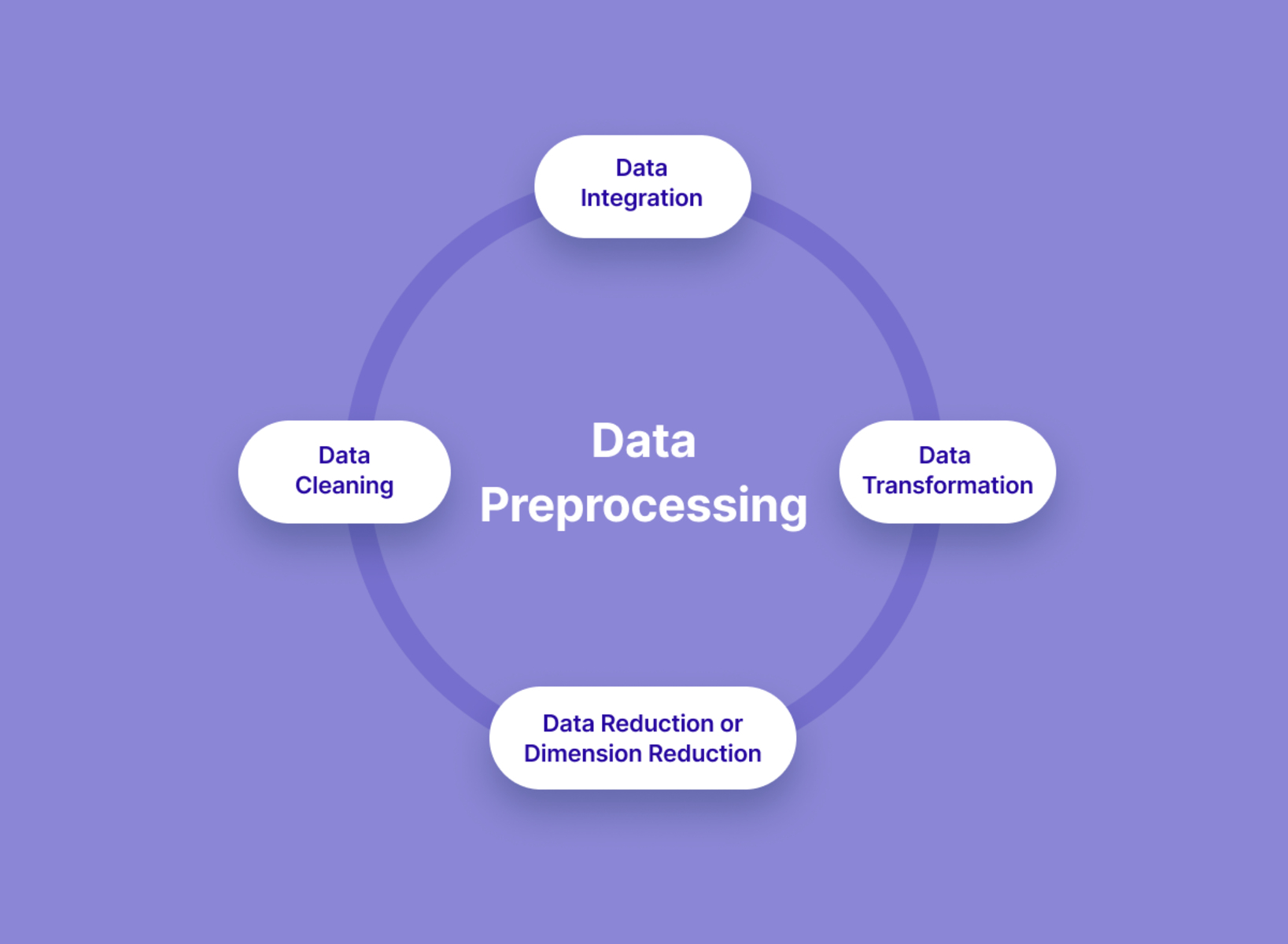
Once we have the data, preprocessing becomes a crucial step. This involves cleaning, transforming, and formatting the data to make it suitable for analysis and modeling. Data cleaning includes handling missing values, removing duplicates, and dealing with outliers that can adversely affect the performance of the models.
Feature engineering is another aspect of data preprocessing that involves creating new features from the existing ones or transforming the features to make them more representative and informative. This can include normalization, scaling, encoding categorical variables, or creating polynomial features. By engineering the features, we can provide the models with the necessary information to make accurate predictions.
Data preprocessing also involves splitting the data into training and testing sets. The training set is used to train the models, while the testing set is used to evaluate their performance. It is important to ensure that the splitting is done randomly and maintains the distribution of the data to ensure reliable evaluation of the models.
In addition to the training and testing sets, it is also a good practice to have a validation set. This subset of data is used for fine-tuning the hyperparameters of the models and preventing overfitting. The validation set helps us choose the best configuration for our models and optimize their performance.
Another crucial step in data preprocessing is handling imbalanced datasets, where the number of instances in each class is significantly different. Techniques such as oversampling the minority class or undersampling the majority class can be used to address this issue and ensure that the models do not favor one class over the others.
By gathering and preprocessing the data, we ensure that the models have access to high-quality, relevant, and representative data. This sets the foundation for accurate and reliable model comparison and evaluation. Proper data preprocessing also helps to address common challenges and biases present in the data, ensuring that the models are robust and generalize well to new, unseen data.
Splitting the Data into Training and Testing Sets
A crucial step in comparing machine learning models is splitting the data into training and testing sets. This ensures that the models are evaluated on unseen data and provides an unbiased assessment of their performance.
The purpose of the training set is to train the models on a subset of the data, allowing them to learn patterns and relationships between the features and the target variable. This enables the models to make predictions when presented with new, unseen data. The training set typically constitutes a large portion of the available data, ensuring that the models have sufficient examples to learn from.
The testing set, on the other hand, is used to evaluate the performance of the models. It consists of data that the models have not seen during the training phase. By evaluating the models on this independent data, we obtain an unbiased assessment of how well the models generalize to new instances.
When splitting the data into training and testing sets, it is important to ensure that the division is done randomly and maintains the distribution of the data. Random splitting helps in reducing bias and ensures that the models are trained and tested on a representative subset of the data.
The commonly used proportions for splitting the data are the 70/30 or 80/20 splits, where 70% or 80% of the data is used for training, and the remaining 30% or 20% is used for testing. However, the specific split ratio may vary depending on the size of the dataset and the specific requirements of the task.
Another approach to splitting the data is k-fold cross-validation. In this method, the data is divided into k equal-sized folds, and the models are trained and tested k times, with each fold serving as the testing set once and the remaining folds as the training set. This approach helps in obtaining a more robust and reliable estimate of the models’ performance.
By splitting the data into training and testing sets, we can objectively assess the performance of the models on unseen data. This ensures that the models are evaluated in a realistic scenario and helps in identifying the model that performs the best in terms of generalization.
In addition to the training and testing sets, it is also common to set aside a validation set. The validation set is used for fine-tuning the hyperparameters of the models and preventing overfitting. It allows us to experiment with different configurations and select the best-performing model before final evaluation on the testing set.
Overall, splitting the data into training and testing sets is a critical step in comparing machine learning models. It allows us to assess their performance objectively and choose the model that best generalizes to new, unseen data.
Training and Fine-Tuning the Models
Once the data is split into training and testing sets, the next step in comparing machine learning models is to train and fine-tune the models on the training data. This process involves optimizing the models’ parameters and finding the best configuration for optimal performance.
Training the models entails feeding the training data into them, allowing them to learn and adjust their internal parameters to minimize the difference between predicted and actual values. The models learn patterns and relationships in the data through an iterative process, improving their ability to make accurate predictions.
During the training process, we need to select an appropriate algorithm or model for the task at hand. Different machine learning algorithms have different characteristics, assumptions, and complexities, making it essential to choose the most suitable one based on the data and problem domain.
As the models are trained, it is crucial to monitor their performance using evaluation metrics such as accuracy, precision, recall, or the chosen metric specific to the problem. This provides insights into how well the models are learning from the training data and helps in identifying potential issues such as underfitting or overfitting.
Underfitting occurs when the model is too simplistic and fails to capture the patterns in the data, resulting in poor performance both on the training and testing sets. Overfitting, on the other hand, happens when the model becomes too complex and ends up memorizing the training data instead of generalizing to new instances. Fine-tuning the models involves experimenting with different hyperparameters to strike the right balance between underfitting and overfitting.
To find the optimal configuration, various techniques can be employed, such as grid search or random search, where different combinations of hyperparameter values are tried and evaluated on a validation set. By systematically exploring the hyperparameter space, we can discover the settings that yield the best performance.
Fine-tuning also involves considering other aspects such as regularization techniques, learning rate, convergence criteria, or ensemble methods. These techniques help in enhancing the models’ ability to generalize and make accurate predictions on unseen data.
By training and fine-tuning the models, we iteratively improve their performance and optimize their configurations. This process allows us to compare the models under fair conditions, ensuring that each model has been adequately trained and optimized to reach its full potential.
It is essential to note that training and fine-tuning the models require computational resources and can be time-consuming, especially for complex models or large datasets. Therefore, it is crucial to carefully plan and allocate the necessary resources and consider the trade-off between computational complexity and model performance.
Once the models are trained and fine-tuned, they are ready for evaluation on the independent testing set. This final evaluation provides a reliable measure of each model’s performance, helping us make an informed decision on the best model for the given task.
Evaluating the Models Using Different Metrics
Comparing machine learning models involves evaluating their performance using various metrics to gain comprehensive insights into their effectiveness and suitability for the task at hand. By assessing models using different metrics, we obtain a holistic understanding of their capabilities and make informed decisions.
One commonly used metric is accuracy, which measures the percentage of correctly classified instances. While accuracy provides a general measure of model performance, it may not be suitable for imbalanced datasets. In such cases, metrics like precision, recall, and F1-score offer more informative evaluations.
Precision represents the proportion of true positive predictions out of all positive predictions made by the model. It conveys the model’s ability to avoid false positive errors. Recall, on the other hand, measures the proportion of true positive predictions out of all actual positive instances. It highlights the model’s capability to find all positive instances. The F1-score combines precision and recall into a single metric, providing a balanced evaluation of model performance.
For certain applications, different metrics may be more appropriate. In binary classification tasks, the area under the receiver operating characteristic curve (AUC-ROC) is commonly used. It considers the trade-off between the true positive rate and the false positive rate, offering a measure of the model’s overall discriminative power.
Other evaluation metrics depend on the specific problem domain and objectives. For instance, in regression problems, mean squared error (MSE) or root mean squared error (RMSE) measure the average squared difference between the predicted and actual values. In recommendation systems, metrics like precision at K or average precision evaluate the relevance of recommended items to users.
It is important to consider multiple metrics to gain a comprehensive understanding of the models’ performance. Each metric reveals a different aspect of the model’s strengths and weaknesses. By evaluating models using multiple metrics, we can identify trade-offs and make more informed decisions based on the specific requirements and goals of the task.
Additionally, visualizing the evaluation results can aid in understanding and interpreting model performance. Techniques such as confusion matrices, ROC curves, and precision-recall curves provide visual representations of the models’ performance across different evaluation metrics. These visualizations contribute to a more intuitive and comparative analysis of the models.
Evaluating models using different metrics allows us to assess their performance comprehensively and objectively. By considering a range of evaluation metrics and visualizing the results, we can gain valuable insights into how well each model performs and make data-driven decisions about the most suitable model for the task.
Comparing the Models Based on Their Performance
Once we have evaluated each machine learning model using various metrics, the next step is to compare the models based on their performance. By comparing the models, we can identify the most suitable one that meets our requirements and achieves the desired outcomes.
One way to compare models is to examine their performance across different evaluation metrics. Considering metrics such as accuracy, precision, recall, F1-score, or AUC-ROC provides insights into the models’ strengths and weaknesses. It allows us to understand how well each model handles different aspects of the task, such as correctly classifying instances, avoiding false positives, or finding all positive instances.
Comparing models goes beyond single metrics, as it involves considering trade-offs and choosing the best compromise. For example, one model may excel in accuracy but lag behind in precision. Depending on the specific requirements of the task, we must decide which metrics are the most valuable and prioritize models accordingly.
It is important to consider the relative performance of the models rather than relying solely on absolute metric values. By comparing models side by side, we can identify which model consistently performs better across multiple metrics or which model excels in specific areas. This comparative analysis guides us in selecting the model that is most suitable for the given task.
Additionally, it is crucial to consider the domain and problem-specific factors when comparing models. Certain models may have characteristics that align better with the nature of the problem or the constraints of the application. For instance, if interpretability is a priority, models such as decision trees may be preferred over more complex models like neural networks, even if the latter achieves higher accuracy.
Furthermore, it is essential to take into account the computational complexity and scalability of the models. Some models may achieve higher accuracy but at the cost of longer training times or increased resource requirements. The decision to prioritize accuracy over efficiency or vice versa depends on the specific constraints and resources available.
By comparing the models based on their performance, taking into account trade-offs, specific requirements, and constraints, we can make an informed decision on which model to choose for the given task. It is important to consider the overall performance, consistency, and suitability of each model to ensure that the chosen model aligns with the desired outcomes and delivers the best performance.
Visualizing the Results
Visualizing the results of comparing machine learning models can greatly enhance our understanding of their performance and aid in making informed decisions. Visualization techniques offer a clear and intuitive representation of how the models perform across different evaluation metrics. They provide insights into the strengths and weaknesses of each model and facilitate the comparative analysis.
One commonly used visualization technique is the confusion matrix. This matrix provides a visual representation of the performance of a classification model by displaying the number of true positives, true negatives, false positives, and false negatives. It allows us to assess the models’ accuracy, precision, recall, and other metrics in a tabular format. Additionally, it provides insights into the specific types of errors the models make, aiding in targeted improvements.
Another powerful visualization tool is the receiver operating characteristic (ROC) curve. The ROC curve illustrates the trade-off between the true positive rate (sensitivity) and the false positive rate (1-specificity) at various classification thresholds. Plotting the ROC curve enables us to compare the models’ discrimination power and choose the one that achieves the best overall performance. Additionally, the area under the ROC curve (AUC-ROC) provides a single metric summarizing the models’ performance and serves as a convenient basis for comparison.
Precision-recall curves are another insightful visualization technique. These curves depict the trade-off between precision and recall at different thresholds. They are particularly useful in imbalanced datasets where precision and recall are more informative metrics than accuracy. Comparing the precision-recall curves allows us to analyze how well the models balance precision and recall and select the model that aligns with the specific requirements of the task.
Beyond these specific visualization techniques, there are numerous other ways to represent and interpret model performance. Bar and line charts, scatter plots, heatmaps, or even interactive visualizations can be used to display the models’ performance across various evaluation metrics or feature importance rankings.
Visualizing the results not only facilitates the comparison of models but also helps in communicating the findings to stakeholders effectively. Visual representations are often more accessible and comprehensible than numerical values alone. This allows for better understanding and collaboration among different stakeholders involved in the decision-making process.
Ultimately, visualizing the results brings an extra layer of clarity and insight to the comparison of machine learning models. It helps us comprehend the performance differences between models, identify areas for improvement, and select the most suitable model for the task at hand.
Considering Algorithm Complexity and Interpretability
When comparing machine learning models, it is crucial to consider the trade-off between algorithm complexity and interpretability. Each model has its own level of complexity and interpretability, and understanding this balance is essential in selecting the most suitable model for a given task.
Algorithm complexity refers to the computational resources and time required to train and deploy the model. Some models, such as deep neural networks or ensemble methods, are inherently more complex and demanding in terms of computational power and data requirements. These models may achieve high accuracy but come at the cost of increased complexity and resource utilization. In contrast, simpler models like linear regression or decision trees are less computationally intensive and relatively easier to understand and implement.
While complexity is important for achieving high accuracy in certain scenarios, it may not always be necessary or practical. It is essential to consider the available resources, including computational power, memory, and the size of the dataset. Choosing a model that strikes the right balance between complexity and the available resources is crucial for practical implementation.
Interpretability, on the other hand, refers to the ability to understand and interpret how the model makes predictions. Some models, such as decision trees or linear regression, provide clear rules and coefficients that can be directly interpreted. These transparent models offer insights into the relationships between the features and the target variable and can be easily explained to stakeholders.
However, as models become more complex, interpretability tends to decrease. Deep learning models, for example, are highly complex and operate in high-dimensional spaces, making it challenging to identify the specific factors driving their predictions. While these models may achieve impressive accuracy, understanding and explaining their inner workings to non-experts can be difficult.
The level of interpretability required depends on the specific application and stakeholders involved. In certain domains, such as healthcare or finance, interpretability is crucial to gain trust, satisfy regulatory requirements, and provide transparent decision-making processes. In other cases, such as image or speech recognition, accurate predictions may take precedence over interpretability.
Therefore, when comparing models, it is important to consider both algorithm complexity and interpretability based on the specific requirements and constraints of the task. Striking the right balance allows us to select a model with the appropriate level of complexity and interpretability, ensuring it aligns with the practical needs and expectations.
By considering algorithm complexity and interpretability, we can make a well-informed decision regarding the best model to use in a specific scenario. This decision requires understanding the resources available, the size and nature of the dataset, and the requirements for interpretability in the context of the problem domain and stakeholders involved.
Making a Final Decision on the Best Model
After evaluating and comparing the machine learning models based on various metrics, considering algorithm complexity, interpretability, and other relevant factors, it is time to make a final decision on the best model for the task at hand.
To make an informed decision, it is important to consider the specific goals and requirements of the project. Each model might have its strengths and weaknesses, and the best model depends on how well it aligns with the project’s objectives. For example, if the primary concern is achieving the highest accuracy, a complex model like a deep neural network may be the appropriate choice. On the other hand, if interpretability and simplicity are key factors, a decision tree or linear regression model might be preferable.
Additionally, the available resources and practical considerations need to be taken into account. Models with higher complexity might require more computational power, memory, or data, which might not be feasible within the project’s constraints. It is important to balance the desired performance with the available resources to ensure practical implementation of the chosen model.
Furthermore, stakeholder preferences and domain-specific requirements also play a role in the decision-making process. Understanding the expectations and needs of stakeholders is crucial in selecting a model that meets their criteria, whether it’s interpretability, ease of implementation, or specific performance metrics.
It is worth considering the robustness and reliability of the selected model as well. Performance on the testing dataset provides an initial measure, but it is important to consider how well the model is expected to generalize to new, unseen data. Techniques such as cross-validation or evaluating the model on independent datasets can provide insights into the model’s ability to handle unforeseen scenarios.
While the decision-making process revolves around objective evaluation, it is also important to acknowledge the inherent uncertainty and imperfections in modeling. No model is perfect, and there is always a degree of uncertainty associated with predictions. Being aware of these limitations helps manage expectations and make decisions based on realistic assumptions.
In summary, making a final decision on the best model involves considering the project’s goals, algorithm complexity, interpretability, available resources, stakeholder preferences, and the model’s robustness. It is a comprehensive evaluation process that balances trade-offs and aligns with the specific requirements of the task at hand. By carefully considering these factors, we can confidently choose the best model that delivers the desired performance and meets the project’s objectives.
Conclusion
Comparing machine learning models is a critical step in selecting the best model for a specific task. By evaluating and considering various aspects such as performance metrics, algorithm complexity, interpretability, and other domain-specific factors, we can make an informed decision.
Throughout this article, we have explored the importance of comparing machine learning models and the steps involved in the process. We have learned about the significance of choosing the right evaluation metrics to assess model performance and the importance of gathering and preprocessing the data. We have also discussed splitting the data into training and testing sets, training and fine-tuning the models, and the process of evaluating the models using different metrics.
Moreover, we have emphasized the need to consider algorithm complexity and interpretability when comparing models. The trade-off between these factors plays a crucial role in determining the most suitable model for a given task. Lastly, we explored the value of visualizing the results to enhance our understanding of the models’ performance and aid in decision-making.
Ultimately, the final decision on the best model depends on a careful consideration of the project’s goals, available resources, specific requirements, and stakeholder preferences. By thoroughly evaluating and comparing the models, we can select the one that achieves the desired outcomes and aligns with the practical constraints of the problem at hand.
As the field of machine learning continues to advance, the availability of various algorithms and techniques provides us with a wide range of options. By following a systematic and thorough approach to comparing and evaluating models, we can leverage the power of machine learning to make accurate predictions, automate tasks, and drive decision-making processes in various domains.
In conclusion, comparing machine learning models is an essential process that enables us to make data-driven decisions and choose the best model for a given task. By understanding the importance of evaluation metrics, data preprocessing, and other considerations, we can confidently select the model that meets our objectives and achieves the best performance.