What Is RL In Machine Learning

Introduction

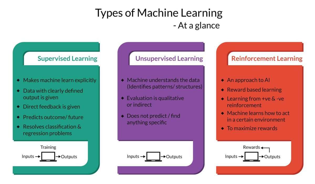
Reinforcement Learning (RL) is a powerful branch of machine learning that focuses on training an agent to make a sequence of decisions in an environment to maximize its cumulative reward. Unlike supervised or unsupervised learning, where the algorithm is provided with labeled or unlabeled data, RL relies on trial and error to learn from the consequences of its actions. This approach makes RL especially well-suited for complex decision-making tasks that have no pre-defined optimal solution.

RL has gained significant attention in recent years due to its ability to tackle difficult problems in various domains. From self-driving cars to robotic control, RL has demonstrated its potential to achieve remarkable results. The key idea behind RL is to learn the optimal policy that determines which actions the agent should take in each state to maximize its long-term rewards.

One of the main challenges in RL is striking the right balance between exploration and exploitation. At the early stages of learning, the agent needs to explore different actions to gather information about the environment. However, as it gathers more knowledge, it should exploit this knowledge to select actions that are likely to yield higher rewards. This trade-off is critical for achieving optimal performance.

RL relies on mathematical models to represent the environment and the agent’s behavior. The Markov Decision Process (MDP) framework is commonly used to formalize RL problems. The agent interacts with the environment by observing a state, taking an action, and receiving a reward. The goal is to find the policy that maximizes the expected cumulative reward.

Reinforcement Learning is not limited to a specific application area. It has been successfully applied to various domains, including game playing, robotics, finance, healthcare, and even in optimizing online advertising campaigns. The versatility of RL makes it an exciting field with tremendous potential for solving complex real-world problems.

In this article, we will explore the fundamental components of reinforcement learning, such as the Markov Decision Process, reward function, state space, action space, policy, and value function. We will also dive into popular algorithms like Q-learning and the Deep Q-Network (DQN). Lastly, we will discuss some of the exciting applications of reinforcement learning in different domains.

What is Reinforcement Learning?

Reinforcement Learning (RL) is a subfield of machine learning that focuses on training an agent to make a sequence of decisions in an environment to maximize its cumulative reward. Unlike supervised learning, where the agent learns from labeled data, or unsupervised learning, where the agent finds patterns in unlabeled data, RL relies on trial and error to learn through interacting with an environment.

In reinforcement learning, the agent is not explicitly told which actions to take but discovers the optimal actions through exploration and exploitation. The agent learns from the consequences of its actions by receiving feedback in the form of rewards or penalties. The ultimate goal of RL is to find the optimal policy, which defines the agent’s strategy in each state, to maximize the expected cumulative reward.

The heart of RL lies in the concept of an agent-environment interaction. The agent interacts with the environment by following a series of steps:

1. The agent observes the current state of the environment.
2. Based on the observed state, the agent selects an action.
3. The agent performs the chosen action, causing a transition to a new state.
4. In response to the action, the agent receives a reward from the environment.
5. The process continues until a terminal state is reached.

The RL agent learns by repeatedly performing these steps, updating its policy based on the observed rewards and transitioning to new states. Through the trial and error process, the agent gradually improves its decision-making capability and learns to make better choices that lead to higher rewards.

Reinforcement Learning is distinct from other types of machine learning in that it does not rely on predefined datasets or explicit knowledge of the environment. RL agents learn through exploration and exploit the knowledge gained to make better decisions. This flexibility makes RL well-suited for solving complex problems that lack a known optimal solution.

Many real-world problems can be framed as RL problems. For example, teaching a robot to navigate a maze, training a self-driving car to navigate city streets, or optimizing the placement of advertisements to maximize user engagement. In each case, the RL agent learns to make decisions based on the feedback it receives from the environment, adapting its strategies to achieve the best possible outcome.

In the following sections, we will delve deeper into the key components of reinforcement learning and explore the algorithms and techniques used to solve RL problems.

The Components of Reinforcement Learning

Reinforcement learning consists of several key components that work together to enable an agent to learn and make informed decisions. Understanding these components is crucial for implementing and solving RL problems effectively. The main components of reinforcement learning include:

Markov Decision Process (MDP): An MDP provides a mathematical framework to model a reinforcement learning problem. It consists of a set of states, a set of actions, transition probabilities, and a reward function. The Markov property assumes that the future state of the environment depends only on the current state and action, making it memoryless.

Reward Function: The reward function defines the goal of the agent. It assigns a numeric value to each state or state-action pair, representing the desirability or utility of that state or action. The agent’s objective is to maximize the cumulative reward over time.

State Space: The state space is the set of all possible states in the environment. It defines the observations that the agent receives at each step. The state space can be discrete, such as a finite set of states, or continuous, represented by a vector of continuous variables.

Action Space: The action space is the set of all possible actions that the agent can take in a given state. Similar to the state space, the action space can be discrete or continuous, depending on the problem domain.

Policy: The policy determines the agent’s decision-making strategy. It defines a mapping from states to actions, specifying which action the agent should choose in each state. The policy can be deterministic, selecting a single action, or stochastic, assigning probabilities to different actions.

Value Function: The value function estimates the expected cumulative reward from a particular state or state-action pair. It provides a measure of the long-term desirability of being in a certain state or taking a specific action. The value function is used by the agent to evaluate and compare different strategies.

By understanding and implementing these components effectively, reinforcement learning agents can learn optimal policies and make decisions that maximize their cumulative rewards. In the next sections, we will explore popular algorithms and techniques used in reinforcement learning, such as Q-learning and Deep Q-Networks (DQN).

Markov Decision Process (MDP)

The Markov Decision Process (MDP) is a mathematical framework used to model reinforcement learning problems. It provides a formal way to describe the interaction between an RL agent and its environment. MDPs are based on the Markov property, which assumes that the future state of the environment depends only on the current state and action, making it memoryless.

In an MDP, the environment is modeled as a sequence of discrete time steps. At each time step, the agent observes the current state of the environment and selects an action to perform. The environment then transitions to a new state based on the chosen action, and the agent receives a reward. This process continues until a terminal state is reached.

The key elements of an MDP include:

• State Space: The state space is the set of all possible states that the environment can be in. It can be discrete or continuous, depending on the problem domain. For example, in a maze navigation problem, the state space could represent different positions in the maze.
• Action Space: The action space is the set of all possible actions that the agent can take in a given state. It can also be discrete or continuous. In the maze navigation problem, the action space could represent different directions the agent can move in (e.g., up, down, left, right).
• Transition Probabilities: The transition probabilities define the likelihood of transitioning to a new state when the agent performs a particular action in a given state. These probabilities can be represented in a transition probability matrix, where each entry corresponds to the probability of transitioning from one state to another.
• Reward Function: The reward function assigns a numeric value to each state or state-action pair. It represents the immediate payoff or desirability of being in a certain state or taking a specific action. The goal of the agent is to maximize the cumulative reward over time.

The MDP framework allows RL agents to reason and plan about their actions in a systematic way. By using dynamic programming algorithms such as value iteration or policy iteration, agents can learn the optimal policy that maximizes the expected cumulative reward. These algorithms iteratively update the value function or policy until convergence is achieved.

MDPs provide a powerful tool for modeling and solving reinforcement learning problems. By defining the state space, action space, transition probabilities, and reward function, the agent can learn to make decisions that lead to the highest achievable reward. In the next section, we will explore the role of the reward function in reinforcement learning.

Reward Function

The reward function is a critical component in reinforcement learning that assigns a numeric value to each state or state-action pair. It represents the immediate payoff or desirability of being in a particular state or taking a specific action. The reward function guides the agent’s decision-making process by providing feedback on the goodness or badness of its actions.

The reward function is designed by the problem designer and plays a vital role in defining the objective of the agent. It quantifies the goals and preferences of the RL problem and determines what the agent should aim to maximize or minimize. The rewards can be positive, negative, or zero, depending on the situation.

When designing a reward function, it is crucial to consider the following factors:

• Goal Alignment: The reward function should be aligned with the desired objective of the RL problem. It should incentivize the agent to reach the desired goal state or perform the desired behavior. For example, in a maze navigation problem, the agent could receive a positive reward for reaching the exit and negative rewards for hitting obstacles.
• Sparse or Dense Rewards: The reward function can be designed to provide rewards at every time step or only when specific goals are achieved. Sparse rewards can make learning more challenging since the agent receives limited feedback. On the other hand, dense rewards can speed up learning and provide more immediate feedback to the agent.
• Balance Exploration and Exploitation: The reward function influences the exploration-exploitation trade-off. If the rewards are too heavily weighted towards immediate gains, the agent might not explore enough to discover more optimal solutions. Finding the right balance between exploration and exploitation is crucial for achieving optimal performance.
• Discounting Future Rewards: In many RL problems, future rewards are discounted to prioritize immediate rewards over delayed rewards. The discount factor, often denoted by gamma (γ), determines the importance of immediate rewards relative to future rewards. A discount factor of 1 means all rewards are considered equally, while a value closer to 0 highlights the importance of immediate rewards.

The reward function shapes the agent’s policy and influences its learning process. Through experience and interaction with the environment, the agent aims to maximize the cumulative reward over the long term. By associating positive rewards with desirable states or actions and negative rewards with undesirable outcomes, the agent learns to make decisions that lead to higher overall rewards.

Designing an effective reward function is a crucial and challenging task in reinforcement learning. It requires careful consideration of the problem domain and the goals of the agent. The reward function lies at the core of the RL agent’s learning process and greatly influences its ability to discover optimal policies. In the next sections, we will explore other components of reinforcement learning, including state space, action space, policy, and value function.

State Space

In reinforcement learning, the state space represents the set of all possible states that the environment can be in. It defines the observations that the RL agent receives at each time step. The state space can be discrete, where only a finite number of states exist, or continuous, represented by a vector of continuous variables.

The state space plays a crucial role in determining the complexity and richness of the RL problem. It encapsulates all the relevant information that the agent needs to make decisions and learn from the environment. The states can include variables such as positions, velocities, sensor readings, or any other relevant information that characterizes the environment’s current condition.

In discrete state spaces, each state represents a unique configuration or situation that the agent can be in. For example, in a chess game, the state space is composed of all possible configurations of the chessboard, including the positions of the pieces. In this case, the state can be encoded as a discrete value, such as a unique number representing a specific board position.

On the other hand, continuous state spaces are characterized by a vector of continuous variables. These variables can be real numbers representing physical quantities, such as position and velocity in a self-driving car or the current stock prices in a financial market. Dealing with continuous state spaces often requires approximation techniques, such as function approximation or discretization, to facilitate learning and decision-making.

Choosing an appropriate state representation is crucial for the success of a reinforcement learning system. The state space should capture all the relevant information needed for the agent to make informed decisions. However, it is equally essential to strike a balance between the richness of the state space and the computational complexity of learning algorithms. An overly complex state space can make learning difficult or computationally intractable.

In some cases, the state space can be indirectly observed, where the agent has access to only partial information about the environment. This is known as a partially observable Markov decision process (POMDP), which requires specialized algorithms to handle the uncertainty and partial observability.

Understanding and modeling the state space is crucial for designing efficient reinforcement learning algorithms. The choice of state representation should consider the complexity of the problem, the available information, and the computational resources. By appropriately defining the state space, the RL agent can learn meaningful representations of the environment and make informed decisions to maximize its cumulative reward.

In the next section, we will explore the action space, which determines the set of possible actions that the agent can take in a given state.

Action Space

In reinforcement learning, the action space refers to the set of all possible actions that an agent can take in a given state. It represents the available choices the agent can make to interact with the environment and influence its future states. The action space can be discrete or continuous, depending on the problem domain.

In a discrete action space, the agent can choose from a finite number of distinct actions. For instance, in a game like chess, the action space is the set of all possible moves that the player can make. Each move represents a unique action that can be taken in a given state.

In contrast, a continuous action space consists of a range of real-valued actions. Examples include controlling the steering angle and acceleration of a self-driving car, or setting the trajectory and speed of a robot arm. Dealing with continuous action spaces often requires specialized algorithms, such as policy gradient methods or Gaussian processes.

The action space can also be constrained, meaning that certain actions are not permissible in specific states. For example, in a board game, there might be rules that restrict certain types of moves depending on the current state of the game. These restrictions need to be taken into account when defining the action space.

The size and complexity of the action space influence the difficulty of the RL problem. As the number of possible actions increases, the agent has more choices to consider, which can make learning and decision-making more challenging. Additionally, in continuous action spaces, finding the optimal action becomes a continuous optimization problem that requires specialized techniques.

In some cases, the action space can change dynamically based on the current state or history of actions. This introduces additional complexity and requires the agent to adapt its decision-making process accordingly.

The exploration-exploitation trade-off, a key challenge in reinforcement learning, is closely related to the action space. The agent needs to balance between exploring new actions to gather information about the environment and exploiting its current knowledge to select actions that are likely to yield high rewards.

Choosing an appropriate action representation is crucial for the success of reinforcement learning algorithms. The action space should be expressive enough to capture meaningful variations in decision-making, while still being feasible to explore and exploit efficiently. Understanding the action space and its constraints is critical for designing effective RL agents.

In the next sections, we will explore the policy, value function, and various algorithms and techniques used in reinforcement learning.

Policy

In reinforcement learning, a policy represents the decision-making strategy of an agent. It defines the mapping between states and actions, determining the action that the agent should take in a given state. The policy guides the agent’s behavior and determines its actions in the environment.

A policy can be deterministic or stochastic. A deterministic policy directly maps states to specific actions without any randomness. For example, in a game of tic-tac-toe, a deterministic policy might dictate that the agent always selects the center square as its first move. Deterministic policies are often used when the environment is predictable and actions have precise outcomes.

On the other hand, a stochastic policy introduces randomness into the decision-making process. It assigns probabilities to different actions in a given state. This randomness allows the agent to explore and learn from its interactions with the environment, promoting a balance between exploration and exploitation.

There are different ways to represent a policy in RL. In some cases, the policy can be explicitly defined as a table or a function that maps states to actions. This is called a tabular policy or a parametric policy, respectively. Other policy representation methods, such as neural networks, can also be used to model complex relationships between states and actions in continuous or high-dimensional state spaces.

Reinforcement learning algorithms aim to find the optimal policy that maximizes the expected cumulative reward. This can be achieved through policy improvement methods, such as policy iteration or policy gradient algorithms. Policy improvement involves iteratively updating the policy based on the observed rewards and transitions, gradually improving the agent’s decision-making capabilities.

The exploration-exploitation trade-off is closely tied to the policy. During the early stages of learning, the agent needs to explore different actions and observe their outcomes to gather information about the environment. As the agent gains experience and knowledge, it can exploit this knowledge to select actions that are likely to lead to higher rewards. Balancing exploration and exploitation is important for the agent to discover optimal strategies while maximizing its cumulative reward.

Designing and updating an effective policy is key to successful reinforcement learning. The choice of policy representation, deterministic or stochastic, and the exploration strategy significantly impact the agent’s learning and decision-making process. By finding the optimal policy, the agent can make informed decisions that maximize its reward in the given environment.

In the following sections, we will explore the value function, Q-learning algorithm, and other popular techniques used in reinforcement learning to further improve decision-making capabilities.

Value Function

In reinforcement learning, the value function is a critical component that assists the agent in evaluating the desirability of states or state-action pairs. It estimates the expected cumulative reward that the agent can achieve from a particular state or state-action pair, providing a measure of the long-term desirability.

There are two primary types of value functions in reinforcement learning:

• State Value Function (V-function): The state value function, denoted as V(s), represents the expected cumulative reward starting from a particular state s. It measures the desirability of being in a certain state and captures the long-term rewards that the agent can achieve from that state. A high state value indicates a more favorable state, while a low value suggests less desirable states.
• Action Value Function (Q-function): The action value function, denoted as Q(s, a), represents the expected cumulative reward starting from a particular state-action pair (s, a). It estimates the value of taking a specific action a in a given state s. The Q-function allows the agent to evaluate the desirability of different actions and select the one that yields the highest expected cumulative reward.

Both the state value function and the action value function play essential roles in reinforcement learning. They provide the agent with a measure of the desirability or quality of states and actions, influencing the agent’s decision-making process.

The value functions can be estimated or learned through various methods, such as dynamic programming, Monte Carlo methods, or Temporal Difference (TD) learning. These techniques update the value functions based on observed rewards and transitions, gradually refining the agent’s understanding of the value of different states and state-action pairs.

By using the value functions, the agent can make informed decisions about which actions to take and which states to aim for. The state value function helps the agent assess the long-term benefits of being in a particular state. On the other hand, the action value function enables the agent to compare the potential rewards of different actions in a given state, aiding in action selection.

The value functions are closely related to the policy of the RL agent. The optimal policy can be derived from the value function by selecting actions that maximize the value. In turn, the value function can be updated using techniques that aim to improve the policy, such as value iteration or Q-learning algorithms.

Understanding and utilizing the value functions effectively is critical for developing successful reinforcement learning algorithms. By estimating the values of states and actions and using them to guide decision-making, the agent can learn optimal strategies and maximize its cumulative reward over time.

In the next section, we will explore the Q-learning algorithm, one of the popular techniques used in reinforcement learning to learn value functions and improve decision-making.

Q-Learning Algorithm

Q-learning is a popular model-free reinforcement learning algorithm used to learn the optimal action value function, also known as the Q-function. It is well-suited for problems where the agent has limited knowledge of the environment and learns solely through interaction.

The Q-learning algorithm utilizes an iterative process to update the Q-values based on the observed rewards and state transitions. The Q-value of a state-action pair (s, a), denoted as Q(s, a), represents the expected cumulative reward when taking action a in state s.

Q-learning employs the following update rule, known as the Bellman equation, to update the Q-values:

Q(s, a) = Q(s, a) + α * (r + γ * max[Q(s’, a’)] – Q(s, a))

In the equation, α (alpha) is the learning rate that determines the weight given to new information, r represents the immediate reward received, γ (gamma) is the discount factor that accounts for the influence of future rewards, and max[Q(s’, a’)] indicates the maximum Q-value among the available actions in the next state s’.

The Q-learning algorithm learns the optimal Q-values by iteratively updating the Q-values for each observed state-action pair. During the learning process, the agent explores the environment by taking actions, receives rewards, and observes the resulting state transitions. The Q-values are updated based on the observed rewards and updated estimates of the next Q-values.

The exploration-exploitation trade-off is crucial in Q-learning. During the early stages of learning, the agent typically follows an exploration strategy, taking random actions to gather information about the environment. As the agent accumulates more knowledge, it tends to exploit the learned Q-values and chooses actions that yield higher expected rewards.

Q-learning is an off-policy algorithm, meaning that it learns the optimal Q-values independent of the policy being followed. This flexibility allows the agent to learn from a mix of exploratory and greedy actions. Additionally, Q-learning is known to converge to the optimal Q-values under certain conditions, guaranteeing the success of the learning process.

The Q-learning algorithm has been successfully applied in various domains, including game playing, robotics, and autonomous systems. It provides a robust and efficient way to learn optimal policies in environments with discrete or continuous state and action spaces.

In the next section, we will explore the Deep Q-Network (DQN), a variant of Q-learning that leverages deep neural networks to learn the Q-function from high-dimensional input spaces.

Deep Q-Network (DQN)

The Deep Q-Network (DQN) is a variant of the Q-learning algorithm that utilizes deep neural networks to approximate the Q-function. DQN is particularly effective in handling high-dimensional state spaces, such as images or sensory data, by learning a meaningful representation of the environment.

In DQN, a deep neural network, often referred to as the Q-network, is used to estimate the Q-values. The Q-network takes the state as input and outputs a Q-value for each possible action. By training the Q-network to approximate the Q-function, DQN enables efficient learning in complex and continuous state spaces.

The training process of DQN involves three key components:

1. Experience Replay: To improve the stability and efficiency of learning, DQN utilizes experience replay. Experience replay involves storing the agent’s experiences, consisting of state, action, reward, and next-state transitions, into a memory buffer. During training, batches of experiences are randomly sampled from the memory buffer, breaking the sequential nature of the data and reducing the correlations between consecutive updates.
2. Target Network: DQN uses a target network that is a separate copy of the Q-network. The target network is used to estimate the target Q-values for training. The weights of the target network are updated less frequently compared to the Q-network, providing a stable target for the updates. This approach mitigates the issue of the Q-values “chasing” each other during the training process.
3. Epsilon-Greedy Exploration: DQN employs an epsilon-greedy exploration strategy to balance exploration and exploitation. The agent randomly selects actions with a probability of epsilon, encouraging exploration, and selects the action with the highest Q-value with a probability of 1 – epsilon, promoting exploitation. By gradually reducing epsilon over time, the agent transitions from exploration to exploitation as it learns more about the environment.

DQN has shown remarkable success in various domains, including playing video games, controlling robotic systems, and managing complex decision-making tasks. It has achieved human-level or even superhuman-level performance in several challenging environments.

One of the advantages of DQN is its ability to handle high-dimensional state spaces, such as images or raw sensory data, without the need for manual feature engineering. The deep neural network automatically learns useful representations, enabling effective decision-making in complex and realistic environments.

While DQN has demonstrated significant success, it also has some limitations. It can be sensitive to hyperparameter settings, and training can be time-consuming due to the need for a large number of samples. Additionally, DQN struggles with problems that have sparse or delayed rewards, as it relies on the observed rewards for updating the Q-values.

Despite these limitations, DQN has proven to be a powerful and versatile algorithm in the field of reinforcement learning. Its success in handling high-dimensional state spaces and achieving impressive performance has paved the way for further advancements in deep reinforcement learning.

In the next sections, we will explore the applications of reinforcement learning in various domains and discuss their real-world impact.

Applications of Reinforcement Learning

Reinforcement Learning (RL) has gained significant attention and has been successfully applied in many domains, demonstrating its potential to tackle a wide range of complex problems. Here are some notable applications of reinforcement learning:

1. Game Playing: Reinforcement learning has achieved remarkable results in game playing. Notably, RL algorithms have defeated human world champions in games like chess, Go, and poker. The ability to learn strategies from scratch and develop sophisticated gameplay makes RL a powerful tool in game AI.
2. Robotics: Reinforcement learning plays a crucial role in robotics, enabling robots to learn to perform tasks and manipulate objects autonomously. RL algorithms have been used to teach robots to walk, grasp objects, and even perform delicate tasks like surgical procedures. The ability to learn from trial and error allows robots to adapt their behavior to different circumstances.
3. Autonomous Vehicles: Reinforcement learning is widely used in autonomous vehicle systems. RL algorithms help vehicles learn how to navigate complex traffic scenarios, make decisions about speed and lane changes, and optimize energy efficiency. RL enables vehicles to learn from real-world experiences and improve their driving performance over time.
4. Resource Management: RL is essential in optimizing resource allocation and management. For example, it is used to control energy consumption in smart grids, optimize inventory management in supply chains, and allocate server resources in cloud computing. RL helps find efficient solutions in dynamic and complex environments.
5. Healthcare: Reinforcement learning has shown promise in healthcare applications. RL algorithms have been used to optimize treatment plans, manage chronic diseases, and develop personalized therapies. The ability to learn and adapt to individual patients’ responses allows for more effective and tailored healthcare interventions.
6. Finance: RL is employed in financial applications, including portfolio management, algorithmic trading, and risk assessment. RL algorithms can learn optimal strategies from historical market data, adapt to changing market conditions, and discover profitable trading opportunities. RL enables intelligent decision-making in dynamic and uncertain financial environments.
7. Natural Language Processing (NLP): RL methods have been successful in NLP tasks, such as language generation, dialogue systems, and machine translation. RL algorithms learn to generate coherent and contextually appropriate responses, enabling more natural and human-like interactions with language-based systems.

These are just a few examples of the diverse applications of reinforcement learning. RL is a versatile and powerful approach that can be adapted to a wide range of domains and problem areas. Its ability to learn from experience and find optimal strategies in complex, uncertain, and dynamic environments makes it an invaluable tool for solving real-world problems.

In the following sections, we will summarize the key points discussed and highlight the potential future developments and challenges in the field of reinforcement learning.

Conclusion

Reinforcement Learning (RL) is a powerful approach to machine learning that focuses on training agents to make sequential decisions in an environment to maximize cumulative rewards. It differs from other types of machine learning by allowing the agent to learn through trial and error rather than relying on labeled data. RL has proven to be successful in a wide range of applications, from game playing and robotics to resource management and healthcare.

The key components of RL, including the Markov Decision Process (MDP), reward function, state space, action space, policy, and value function, work together to enable agents to learn optimal decision-making strategies. Reinforcement learning algorithms, such as Q-learning and Deep Q-Networks (DQN), provide systematic methods for updating policies and estimating the value functions.

Reinforcement learning has shown tremendous potential, especially in complex and dynamic environments. It is particularly well-suited for problems that lack a pre-defined optimal solution or require real-time decision-making. RL enables agents to adapt and learn from their interactions with the environment, continually improving their performance over time.

However, reinforcement learning is not without its challenges. It often relies on exploration to gather information, which can be time-consuming and resource-intensive. Balancing exploration and exploitation is crucial for efficient learning. Additionally, RL algorithms can struggle with sparse rewards or high-dimensional state spaces, requiring careful algorithm design and specialized techniques like function approximation or deep neural networks.

Despite these challenges, the field of reinforcement learning continues to advance rapidly. Researchers are exploring new algorithms, such as model-based reinforcement learning and actor-critic methods, to tackle more complex and diverse problems. Deep reinforcement learning, combining RL with deep neural networks, has shown remarkable success and opened up new possibilities in handling high-dimensional data.

In conclusion, reinforcement learning is a fascinating field with significant potential for solving complex decision-making problems. With its ability to learn by interacting with the environment and optimize long-term rewards, RL continues to find applications in various domains and contribute to advancements in artificial intelligence.